The Bayesian Network Profound Meaning

11 Jul 2018

Prologue To The Bayesian Network Profound Meaning

Bayesian networks(BNs), also known as belief networks(or Bayes nets for short), belong to the family of probabilistic graphical models(GMs), which are used to represent knowledge about an uncertain domain. BNs combine principles from graph theory, probability theory, computer science, and statistics.

Explaining Away

[1] Recap: d-separation

Accordingly, when one set of random variables, $\Theta_{1}$, is conditionally independent of another, $\Theta_{2}$, given a third, $\Theta_{3}$, then we say that the random variables in $\Theta_{1}$ are d-separated from $\Theta_{2}$ by $\Theta_{3}$. For the simplicity, you can treat each set containing only one random variable.

[2] Illustration of explaining away

Given that you got a headache, there exists more than a dozen of possible causes, the causal relationship is depicted below.
➀suppose the inferred correct root cause to your headache is the nasal congestion.
➁the possibility of the rest nodes to be the root cause is greatly reduced, said they has been explained away.
➂given the evidence of a headache, some knowledge of food poisoning, caffeine, alcohol, faulty posture would be inferred from the state of nasal congestion and the observation of a headache.
➃they are no longer d-separated, but d-connected. Or they are conditionally dependent given a headache.

[3] Conclusion

D-connection in converging type networks requires some knowledge of the connection variable(the headache node in this example), at least one of the descendants, the observed evidence must have the positive or the negative information.

The Markov Blanket And Markov Equivalence

[1] Markov blanket

The Markov blanket claims a node is conditionally independent(d-separated) from all of the other nodes(entire graph), given its parents, childs, child's parents.
➀in above graph, given nodes $C$, $D$, $E$, $F$, $G$, node $X$ is d-separated from all othere nodes, $A$, $B$, $H$, $I$, $J$.
➁the parents, the children, other parents of a node's children are called the Markov blanket of a node.
➂therefore Markov blanket contains all the variables that shields the target node from the rest of the network. This means that the Markov blanket of a target node is the only knowledge needed to predict the behavior of that target node.

Suppose we know the value of each node in the Markov blanket, if we’d like to predict the probability distribution of $X$, then there is no more information regarding to the value taken by the node $X$.

[2] Markov equivalence

Two DAGs are to be said Markov equivalent, if they have the same d-separations.

Prove The Markov Blanket

A node is conditionally independent of all other nodes given its Markov blanket, i.e. its parents, its children, and parents of common children(spouses).

proof::mjtsai1974

By using the same DAG of Markov blanket:
➀given target node’s parent, the target node is conditionally independent from the parent’s ascendant. $X$ is d-separated from $A$, given $C$ or $D$.
➁knowing $A$ could predict $C$, then from $C$ to predict $X$; knowing $X$ could infer $C$, then from $C$ to infer $A$. But, knowing $X$ helps nothing in inferring $A$, if we already know $C$; knowing $A$ makes no prediction about $X$, if we already know $C$.
➂given target node’s children, the target node is conditionally independent from the children’s descendants. $X$ is d-separated from $H$, given $F$, and is d-separated from $I$, $J$, given $G$. Similar in ➀.
➃given target node’s children, the children’s parent, the target node would be explained away, the same for that children’s parent, depends on the information on that children.
➄continue on, given $E$, $G$ is d-separated from $B$, then $X$ is also d-separated from $B$.

Therefore, the Markov blanket contains everything we need to predict and infer the target node.

Bayes Theorem With Background Context

[1] Incorporating the background context

Below is an intuitive Bayesian network:
We can deduce the posterior by incorporating the background context in the Bayes theorem expression:
$\;\;P(H\vert E,C)$=$\frac {P(E\vert H,C)\cdot P(H\vert C)}{P(E\vert C)}$

➀$C$, the background context.
➁$P(H\vert C)$, the hypothesis or prior term, based on the background context.
➂$P(E\vert H,C)$, the likelihood term, for the evidence, given the hypothesis and the background context.
➃$P(E\vert C)$, the total probability of evidence given the background context, and is independent of the hypothesis. It is the normalizing or scaling factor.
➄$P(H\vert E,C)$, the posterior term, the belief in hypothesis given evidence and the background context.

[2] Update probabilities of Bayesian network

In my prior post The Bayesian Inference Exploitation, I have exploited the process to update the prior(hypothesis) from the posterior.

New information about one or more nodes in the network updates the probability distributions over the possible values of each node. There are two ways in which information can propagate in a Bayesian network:
➀predictive propagation, it is straightforward, just by following the direction by the arrows. Once new information changes the probability of a node, the node will pass the information to its children, which in turn pass to its children, and so on.
➁retrospective propagation, it is an inverse of predictive propagation. Under retrospective propagation, when a node is updated, it will pass the information to its child node. But, if it is updated from the childe node, the information is passed to its parent node, and in turn pass to its parent node, and so on.

You can think of the update of information from one node to another is simultaneous(maybe atomic), if one node has multiple children, or parents.

Factorization In Bayesian Network

[1] Definition of DAG

According to the Introduction into Bayesian networks, p.6, Mgr. Libor Vaněk, we can define DAG as $G$=$(V,E)$, $V$ for the set of indices to random variables, $E$ for the edges, and $X$=$\{X_{v}: v\in V\}$ to be the set of random variables indexed by $v$.

[2] Factorization definition

$X$ is a Bayesian network with respect to $G$, if the model’s full joint probability density function could be expressed as a product of a series of the random variables’ PDFs(probability density functions), with each PDF having its probability conditionally depending on its parents:
$\;\;P(X)$=$\prod_{v\in V}P(X_{v}\vert pa(X_{v}))$, where $pa(X_{v})$ is the set of parents of $X_{v}$.

[3] Compare chain rule with conditional independence

Suppose $X$ has $n$ nodes in its network:
➀$P(X_{1}=x_{1},…,X_{n}=x_{n})$…by chain rule
=$\prod_{v=1}^{n}P(X_{v}=x_{v}\vert X_{v+1}=x_{v+1},…,X_{n}=x_{n})$
=$P(X_{1}=x_{1}\vert X_{2}=x_{2},…,X_{n}=x_{n})$
$\;\;\cdot P(X_{2}=x_{2}\vert X_{3}=x_{3},…,X_{n}=x_{n})$
$\;\;…$
$\;\;\cdot P(X_{n-1}=x_{n-1}\vert X_{n}=x_{n})$
➁$P(X_{1}=x_{1},…,X_{n}=x_{n})$…by factorization
=$\prod_{v=1}^{n}P(X_{v}\vert (X_{i1},X_{i2},X_{i3},…))$
; where $pa(X_{v})$=$\{X_{i1},X_{i2},X_{i3},…\}$

These 2 expressions differ in that the factorization of conditional independence for any descendant takes only its parents as the conditioning events, as I have shown it in the section “The Joint Probability Distribution Of Bayesian Network” in Introduction To The Bayesian Network.

Example: The Possible Causes To Computer Failure

This is an example from Bayesian networks, Michal Horný, Technical Report No. 5, April 18, 2014, which in turn simplified from Cowel et al, (1999). This example is illustrated here provided that I have a full implementation and explaination with the consistent result.

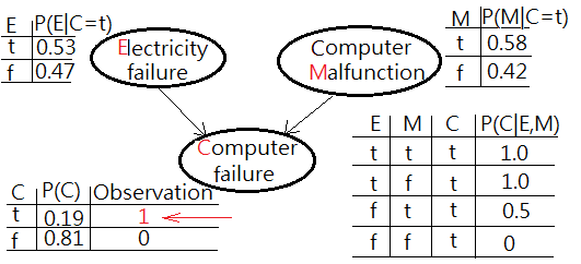
[Scene 1: the prior probability distribution, before evidence]

We are given a question of infering the possible root cause of computer failure(M), suppose the experiment comes with two possible suspects, electricity failure(E), computer malfunction(C):
➀the given prior, $P(E)$, $P(M)$ and the likelihoods of $P(C=t\vert E,M)$ are exhibited with the estimated probability for computer failure, $P(C)$ in below graph.
➁$P(C=t)$
=$\sum_{E,M}P(C\vert E,M)\cdot P(E,M)$
=$\sum_{E,M}P(C\vert E,M)\cdot P(E)\cdot P(M)$
=$1\cdot 0.1\cdot 0.2$+$1\cdot 0.1\cdot 0.8$+$0\cdot 0.9\cdot 0.8$+$0.5\cdot 0.9\cdot 0.2$
=$0.02$+$0.08$+$0$+$0.09$
=$0.19$…the estimated probability of computer failure

[Scene 2: the posterior probability distribution, after evidence]

Assume we have been updated by the observation of physical computer failure, by the retrospective propagation, we could infer the possible root cause from the evidence.
➀$P(E=t\vert C=t)$
=$\sum_{M}P(E=t,M\vert C=t)$
=$\frac {\sum_{M}P(C=t\vert E=t,M)\cdot P(E=t)\cdot P(M)}{P(C=t)}$
=$\frac {1\cdot 0.1\cdot 0.2+1\cdot 0.1\cdot 0.8}{0.19}$
=$0.526315789$
$\approx 0.53$
➁$P(M=t\vert C=t)$
=$\sum_{E}P(M=t,E\vert C=t)$
=$\frac {\sum_{E}P(C=t\vert E,M=t)\cdot P(E)\cdot P(M=t)}{P(C=t)}$
=$\frac {1\cdot 0.1\cdot 0.2+0.5\cdot 0.9\cdot 0.2}{0.19}$
=$0.578947368$
$\approx 0.58$

The posterior of $P(M=t\vert C=t)$ is greater than $P(E=t\vert C=t)$ has been inferred by the observed evidence and depicted in below graph.

Example: The Possible Causes To Computer Failure And Light Failure

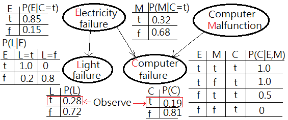
Extended from above example with one extra node of light failure(L) added in the network, conditionally dependent on electricity failure.

[Scene 1: the prior probability distribution, before evidence]

➀the given prior, $P(E)$, $P(M)$ and the likelihoods of $P(C=t\vert E,M)$, $P(L=t\vert E)$ are exhibited with the estimated probability for computer failure, $P(C)$, light failure, $P(L)$ in below graph. ➁$P(L=t)$
=$\sum_{E}P(L=t\vert)\cdot P(E)$
=$0.1\cdot 1.0+0.9\cdot 0.2$
=$0.28$…the estimated probability of light failure

[Scene 2: the posterior probability distribution, after evidence]

Assume we have been updated by the observation of physical computer failure and light failure, by the retrospective propagation, we could infer the possible root cause from the evidence.

Cautions must be made that the probability distribution and its expression has been changed as a result that the network has been new added a node. This is to ask for $P(E=t\vert C=t,L=t)$ and $P(M=t\vert C=t,L=t)$. I am going to take the advantage of factorization in the full joint joint PDF of this model:

➀$P(E=t\vert C=t,L=t)$=$\frac {E=t,C=t,L=t}{P(C=t,L=t)}$
,and $P(M=t\vert C=t,L=t)$=$\frac {M=t,C=t,L=t}{P(C=t,L=t)}$, for the commonality, we should deduce out the full joint PDF.
➁$P(E,M,C,L)$
=$P(L\vert E)\cdot P(C\vert E,M)\cdot P(E)\cdot P(M)$
➂$P(E=t,C=t,L=t)$
=$\sum_{M}P(E=t,M,C=t,L=t)$
=$P(L=t\vert E=t)\cdot P(C=t\vert E=t,M)\cdot P(E=t)\cdot P(M)$
=$1\cdot1\cdot 0.1\cdot 0.2+1\cdot 1\cdot 0.1\cdot 0.8$
=$0.1$
➃$P(C=t,L=t)$
=$\sum_{E}\sum_{M}P(E,M,C=t,L=t)$
=$\sum_{E}\sum_{M}P(L=t\vert E)\cdot P(C=t\vert E,M)\cdot P(E)\cdot P(M)$
=$1\cdot 1\cdot 0.1\cdot 0.2$
$\;\;$+$1\cdot 1\cdot 0.1\cdot 0.8$
$\;\;$+$0.2\cdot 0.5\cdot 0.9\cdot 0.2$
$\;\;$+$0.2\cdot 0\dot 0.9\cdot 0.8$
=$0.118$
➄$P(E=t\vert C=t,L=t)$
=$\frac {E=t,C=t,L=t}{P(C=t,L=t)}$
=$\frac {0.1}{0.118}$
=$0.847457627$
$\approx 0.85$
➅$P(M=t,C=t,L=t)$
=$\sum_{E}P(M=t,M,C=t,L=t)$
=$\sum_{E}P(L=t\vert E)\cdot P(C=t\vert E,M=t)\cdot P(E)\cdot P(M=t)$
=$1\cdot 1\cdot 0.1\cdot 0.2+0.2\cdot 0.5\cdot 0.9\cdot 0.2$
=$0.038$
➆$P(M=t\vert C=t,L=t)$
=$\frac {M=t,C=t,L=t}{P(C=t,L=t)}$
=$\frac {0.038}{0.118}$
=$0.322033898$

The posterior of $P(E=t\vert C=t,L=t)$ is greater than $P(M=t\vert C=t,L=t)$ has been inferred by the observed evidence and depicted in below graph.

Addendum

➀Bayesian networks, Michal Horný, Technical Report No. 5, April 18, 2014
➁Bayesian Networks, Ben-Gal Irad, in Ruggeri F., Faltin F. & Kenett R., Encyclopedia of Statistics in Quality & Reliability, Wiley & Sons (2007).
➂Introduction to discrete probability theory and Bayesian networks, Dr. Michael Ashcroft, September 15, 2011
➃Markov blanket
➄What are Bayesian belief networks?(part 1)
➅Introduction into Bayesian networks, Mgr. Libor Vaněk
➆Cowel R. G., Dawid A. P., Lauritzen S. L., Spiegelhalter D. J. (1999): Probabilistic Networks and Expert Systems. Springer-Verlag New York. ISBN 0-387-98767-3.