Variable Elimination Order And Moral Graph

29 Jul 2018

Prologue To Variable Elimination Order And Moral Graph

The Bayesian network is a DAG(directed acyclic graph), while the moral graph is an undirected version, also known as the Markov network. The moral graph could facilitate the explanation of the factorization in variable elimination process and its order.

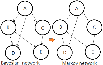
Moral Graph Of A BN(Bayesian Network)

[The moralization algorithm]

➀drop the connectivity in the original Bayesian network, that is to remove the arrow from the arc.
➁connect the parents that shares a common child, that is to marry them.

The resulting undirected graph is the moral graph of a Bayesian network.

This undirected graph is also named Markov network.

The Markov network encodes the CPD in the Bayesian network as a factor of all related variables, like $P(E\vert B,C)$ is expressed in a factor form, $f(B,C,E)$, related variables in each distinct CDP are now be connected by an edge.

[Question]

Why we turn the CDP in the Bayesian network into the factorized form in the Markov network?

[Answer]

Because the moral graph is undirected, it is not in conditionally distributed, rather than, in joint distributed!!

I-Map(Independence Map)

[Definition]

Given below 2 prerequisites:
➀let $I(G)$ be the set of all conditional independences implied by the DAG, said $G$.
➁let $I(P)$ be the set of all conditional independences that holds for or belongs to the joint probability distributiuon, said $P$.

We define the DAG $G$ is an I-Map of a distribution $P$, if $I(G)\subseteq I(P)$.

[Full connected DAG]

A fully connected DAG $G$ is an I-Map for any probability distribution, since:
$I(G)$=$\varnothing\subseteq I(P)$ for all $P$

[Minimal I-Map]

$G$ is a minimal I-Map for P, if any removal of a single edge makes it not an I-Map.
➀a joint probability distributrion might have multiple minimal I-Maps.
➁each corresponds to a specific node-ordering.

[Perfect map]

For $I(G)$=$I(P)$, we say $G$ is a perfect map for $P$.

This section could be found at Probabilistic graphical models, David Sontag, New York University, Lecture 2, February 2, 2012, p.5

Concept Of Potentials

[1] What is a potential?

A potential $\phi_{\chi}$ over a set of random variables $\chi$ is a function that maps each combination of configurations to a non-negative real number.

The conditional probability distribution, joint probability distribution are all the special cases of potential. The domain of a potential $\chi$ is denoted as:
$dom(\phi_{\chi})$=$\chi$

[2] Moralizing and domain graph

Let $\phi$=$\{\phi_{1},\phi_{2},…,\phi_{n}\}$ to be the potentials over a set of random variables, $\chi$=$\{X_{1},…,X_{m}\}$, and with its domain distributed as $dim(\phi_{i})$=$D_{i}$.
➀the domain graph for $\phi$ is the undirected graph with random variables $X_{1}$,…,$X_{m}$ as nodes and link exists between node pairs belonging to the same domain.
➁it is also known as moral graph.

[3] Potential and its domain

Given that $\phi$=$\{\phi_{1},…,\phi_{5}\}$ is a set of potentials over $\{X_{1},…,X_{5}\}$, below graph exhibits the potential with respect to its domain:
, where $\phi_{1}$=$P(X_{1})$,$\phi_{2}$=$P(X_{2}\vert X_{1})$,$\phi_{3}$=$P(X_{3}\vert X_{1})$,$\phi_{4}$=$P(X_{4}\vert X_{2},X_{3})$,$\phi_{5}$=$P(X_{5}\vert X_{4})$.

[4] The fill-ins

In variable elimination process, the removal of one variable would possibly generate a new potential over a domain that didn't exist in the original domain graph, such new potential is the fill-in.
The goal of the most optimal variable elimination sequence is to introduce no extra fill-ins.

Factorization In MN(Markov Network)

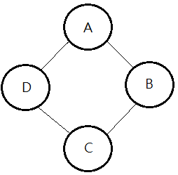
[1] The full/joint PDF in MN

Given below MN, base on our concept that potential is a CPD or a factor of joint distribution, then:
➀$P(A,B,C,D)$…joint PDF
=$\frac {1}{Z}\cdot\phi_{1}(A,B)\cdot\phi_{2}(B,C)\cdot\phi_{3}(C,D)\cdot\phi_{4}(D,A)$
➁Z..normalization factor
=$\sum_{A,B,C,D}\phi_{1}(A,B)\cdot\phi_{2}(B,C)\cdot\phi_{3}(C,D)\cdot\phi_{4}(D,A)$
also called the partition function.

[2] Tight relation between factorization and independence

$X\perp Y\vert Z$ iff $P(X,Y,Z)$=$\phi_{1}(X,Z)\cdot\phi_{2}(Y,Z)$,
then, $(A\perp C\vert D,B)$ and $(B\perp D\vert A,C)$.

proof::mjtsai1974

To show $(A\perp C\vert D,B)$’s independence:
➀$P(A,C,D,B)$=$\psi_{1}(A,D,B)\cdot\psi_{2}(C,D,B)$
, where $\psi_{i}$ is the potential.
➁for $\psi_{1}(A,D,B)$’s independence:
$B\perp D\vert A$
$\Leftrightarrow P(B,D,A)$=$\phi_{1}(B,A)\cdot\phi_{4}(D,A)$
➂for $\psi_{2}(C,D,B)$’s independence:
$B\perp D\vert C$
$\Leftrightarrow P(B,D,C)$=$\phi_{2}(B,C)\cdot\phi_{3}(D,C)$
➃$P(A,C,D,B)$
=$\phi_{1}(B,A)\cdot\phi_{2}(B,C)\cdot\phi_{3}(D,C)\cdot\phi_{4}(D,A)$

$(B\perp D\vert A,C)$’s independence could be proved in similar way.

[3] Factors in MN

A factor can below representations:
➀a joint distribution over $D$ by defining $\phi(D)$.
➁a CPD $P(X\vert D)$, by defining $\phi(X\cup D)$

Factors in MN is a more symmetric parameterization that captures the affinities in between related random variables.

The Gibbs Distribution For BN Versus MN

[1] The Gibbs distribution

A distribution $P_{\phi}$ is a Gibbs distribution if it parameterizes a set of factors $\phi(D_{1})$,…,$\phi(D_{m})$ in the expression:
$\;\;P_{\phi}(X_{1},…,X_{n})$=$\frac {1}{Z}\cdot\phi(D_{1})\cdot\cdots\cdot\phi(D_{m})$, where:
➀$X_{1},…,X_{n}$ are the random variables, $\phi(D_{1}),…,\phi(D_{m})$ are the factors over domains grouped by the related variables and $D_{i}$’s are the domains.
➁$Z$…partition function
=$\sum_{X_{1},…,X_{n}}\phi(D_{1})\cdot\cdots\cdot\phi(D_{m})$
➂a factor is one contribution on the joint operation in variable elimination process.
➃a distribution $P_{\phi}$ with $\phi(D_{1})$,...,$\phi(D_{m})$ factorizes a Markov network if each $\phi_{i}$ is a complete subgraph of it.

[2] The independence in MN

Given this network, we’d like to prove $A\perp C\vert B$ given $P(A,B,C)$=$\frac {1}{Z}\cdot\phi_{A,B}(A,B)\cdot\phi_{B,C}(B,C)$:

proof::mjtsai1974

➀$P(a\vert c)$
=$\frac {P(a\cap c)}{P(c)}$
=$\frac {\sum_{b}P(a,b,c)}{\sum_{a,b}P(a,b,c)}$
=$\frac {\sum_{b}\phi_{A,B}(a,b)\cdot\phi_{B,C}(b,c)}{\sum_{a,b}\phi_{A,B}(a,b)\cdot\phi_{B,C}(b,c)}$
=$\frac {\phi_{A,C}(a,c)}{\phi_{C}(c)}$
It is evident $A$ is independent from $C$ and could be figured out by factors of $A$ and $C$.
➁$P(a\vert b)$
=$\frac {\sum_{c}P(a,b,c)}{\sum_{a,c}P(a,b,c)}$
=$\frac {\sum_{c}\phi_{A,B}(a,b)\cdot\phi_{B,C}(b,c)}{\sum_{a,c}\phi_{A,B}(a,b)\cdot\phi_{B,C}(b,c)}$
=$\frac {\phi_{A,B}(a,b)\cdot\sum_{c}\phi_{B,C}(b,c)}{\sum_{a}\phi_{A,B}(a,b)\cdot\sum_{c}\phi_{B,C}(b,c)}$
=$\frac {\phi_{A,B}(a,b)}{\sum_{a}\phi_{A,B}(a,b)}$
It is evident that the relationship of $A$ and $B$ is estimated by only factor of $A$ and $B$.
➂$P(a,c\vert b)$
=$\frac {P(a,b,c)}{P(b)}$
=$\frac {\phi_{A,B}(a,b)\cdot\phi_{B,C}(b,c)}{\sum_{a,c}\phi_{A,B}(a,b)\cdot\phi_{B,C}(b,c)}$
=$\frac {\phi_{A,B}(a,b)\cdot\phi_{B,C}(b,c)}{\sum_{a}\phi_{A,B}(a,b)\cdot\sum_{c}\phi_{B,C}(b,c)}$
=$\frac {\phi_{A,B}(a,b)}{\sum_{a}\phi_{A,B}(a,b)}\cdot\frac {\phi_{B,C}(b,c)}{\sum_{c}\phi_{B,C}(b,c)}$
=$P(a\vert b)\cdot P(c\vert b)$
This evidence is more confident in our deduction result!! By ➀, ➁, we can conclude that the probability of a variable conditioned on its Markov blanket depends only on potentials involving that node.

[3] BN with evidence is Gibbs in MN

➀suppose you are given a Bayesian network over $\chi$=$\{A,B,C,D,E\}$ illustrated in this graph, where we have the full joint PDF as:
$P_{\chi}(A,B,C,D,E)$
=$P(E\vert C)\cdot P(D\vert B,C)$
$\;\;\cdot P(B\vert A)\cdot P(C\vert A)\cdot P(A)$
➁given the observation of $e$ on node $E$, then:
$P(a,b,c,d\vert E=e)$
=$\frac {P(a\cap b\cap c\cap d\cap e)}{P(e)}$
=$\frac {P(e\vert c)\cdot P(d\vert b,c)\cdot P(b\vert a)\cdot P(c\vert a)\cdot P(a)}{\sum_{A,B,C,D}P(A,B,C,D,e)}$
Evidently, this is a Gibbs distribution!!
➂we moralize the BN by connecting nodes $B$ and $C$ for they are parents of node $D$, and we have potentials thus expressed:
$\phi_{\chi}(A,B,C,D,E)$
=$\frac {\phi_{A,B,C}(A,B,C)\cdot\phi_{B,C,D}(B,C,D)\cdot\phi_{C,E}(C,E)}{\sum_{A,B,C,D,E}\phi_{A,B,C}(A,B,C)\cdot\phi_{B,C,D}(B,C,D)\cdot\phi_{C,E}(C,E)}$
, where $\phi_{A,B,C}(A,B,C)$=$\phi_{A,B}(A,B)\cdot\phi_{A,C}(A,C)\cdot\phi_{A}(A)$
➃given the observation of $e$ on node $E$, then:
$\phi(a,b,c,d\vert e)$
=$\frac {\phi_{\chi}(a,b,c,d,e)}{\phi(e)}$
=$\frac {\phi_{A,B,C}(a,b,c)\cdot\phi_{B,C,D}(b,c,d)\cdot\phi_{C,E}(c,e)}{\sum_{A,B,C,D}\phi_{A,B,C}(A,B,C)\cdot\phi_{B,C,D}(B,C,D)\cdot\phi_{C,E}(C,e)}$
Surprisingly, a Gibbs distribution again!!
We can conclude that any BN conditioned on evidence can be regarded as a Markov network.

Variable Elimination From BN To MN

Still using the same example in Prof. Abbeel, steps through a few variable examples for the illustration with a mapping of each step from BN to MN.
To speed up the path to $P(U\vert +z)$, I use the optimal order of elimination: $W$,$Y$,$X$,$V$
➀eliminate the node $W$.
➁eliminate the node $Y$.
➂eliminate the node $X$.
➃eliminate the node $V$.
➄therefore, we have:
$P(U\vert +z)$
=$\frac {f_{4}(+z,U)\cdot P(U)}{\sum_{u}f_{4}(+z,u)}$
=$\frac {\phi_{Z,U}(+z,U)\cdot\phi_{U}(U)}{\sum_{u}\phi_{Z,U}(+z,u)}$

We conclude that each elimination in BN could be well expressed in terms of potentials in MN.

Addendum

➀Variable elimination, CS228, Stefano Ermon
➁Probabilistic graphical models, David Sontag, New York University, Lecture 2, February 2, 2012
➂Bayesian networks and decision graphs, F.V.Jensen, Springer-Verlag New York, 2001
➃Probabilistic graphical models, Raquel Urtasun and Tamir Hazan, TTI Chicago, April 4, 2011
➄From Bayesian networks to Markov networks, Sargur Srihari