The Calibrated Clique Tree

12 Nov 2018

Prologue To The Calibrated Clique Tree

The quantitative evaluation of messages from one clique to its adjacent clique and from this adjacent clique to itself would be a equilibrium in a calibrated clique tree.

Before We Go Any Farther

[1] Recap: variable-elimination constructed clique tree

Remember that my prior post The Clique Tree Construction has proved that slight different and very different elimination order constructed clique tree makes the same propagation.

[2] Recap: message passing in the clique tree

Still in another prior post of mine, The Bayesian Network Propagation And Clique Tree:
➀the message propagation in the clique tree is proceeded in two stage operations with the former the collection(from leaf nodes to the pivot node) and the next is the distribution(from pivot node to the leaf nodes).
➁computation sharing in all queries that the function of the message from the pivot to the leafs are all expressed in terms of the variables the same as it is in the clique from which passes message to the pivot.
➂given clique $C$ and $C’$ in adjacent, there exists $C_{i}$ for $i$=$1$ to $k$ to be $C$’s neighbors, $g_{i}$ is the message from $C_{i}$ to $C$, and $f_{j}$ is the $j$-th function attached to clique $C$, the message from $C$ to $C’$ is denoted as $H$, expressed as:
$H((C\cap C’)-E)$=$\sum_{C\backslash C’\cup E}\prod_{i}g_{i}\prod_{j}f_{j}$, with $E$ to be the evidence.

The summation over elements purely from $C$

, not belonging to $C’$ and $E$(evidence), then:
$H((C\cap C’)-E)$=$\sum_{C\backslash C\cap C’}\prod_{i}g_{i}\prod_{j}f_{j}$ also holds for it sums out the variables only in $C$!! The term $(C\cap C’)-E$ illustrates that the message purely propagates from $C$ to $C’$, exclusive of the intermediate noise.

[3] Notes

The clique tree is also called a junction tree or a join tree.

What Is The Calibrated Clique Tree?

[1] Run message passing with each clique in the tree as the pivot(root)

Suppose you have a well constructed clique tree:
➀take one clique that neither has been used as a pivot nor all its containing variables has been belief updated.
➁run message passing from leave nodes to this pivot node with one variable chosen for belief update(such variable must not have been propagated with message in this clique).
➂in the message passing from one clique to another, marginalizes over variables other than ➁ chosen variable, thus to have the final factor containing only this variable in it.
➃repeat ➀ until each clique and all variables in it has been belief updated.

[2] The calibrated clique tree

After each clique with all its variables has been belief updated, we will have a calibrated clique tree if below condition is satisfied:
$\;\;\sum_{C_{i}\backslash S_{i,j}}Bel_{i}$=$\sum_{C_{j}\backslash S_{i,j}}Bel_{j}$
where,
➀we denote $Bel_{i}$ for the belief update on clique $i$.
➁we take $S_{i,j}$=$C_{i}\cap C_{j}$ as the edge in between $C_{i}$ and $C_{j}$.
➂$C_{i}$ and $C_{j}$ are any two adjacent cliques in the tree.
➃we say that $C_{i}$ and $C_{j}$ are calibrated.

We can also use $Bel_{i}(X)$ to be the posterior belief update of variable $X$ in clique $i$; for the simplicity, the belief update would be proceeded in the unit of each distinct clique in this article.

Illustrtation Of The Calibrated Clique Tree::by mjtsai1974

[1] From BN to MN

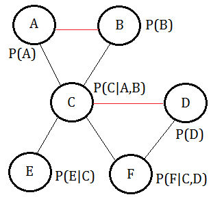
Suppose we are given this BN, with probability distributed over each variable:
➀the total joint probability would be
$P(A,B,C,D,E,F)$
=$P(F\vert C,D)\cdot P(E\vert C)\cdot P(D)$
$\;\;P(C\vert A,B)\cdot P(B)\cdot P(A)$
➁we’d like to query for $P(A,B,C\vert d,e,f)$=$\frac {P(A,B,C,d,e,f)}{\sum_{A,B,C}P(A,B,C,d,e,f)}$, under the observation(evidence) that $D$=$d$,$E$=$e$,$F$=$f$.
➂moralize it, we get below MN.

[2] Construct the clique tree

By using the variable elimination order $A,B,E,F,D,C$, we construct this clique tree:
➀we choose the clique $(A,B,C)$ as the pivot, for the 1st phase of collection:
$f_{2}(C)$=$\sum_{E}P(E\vert C)$
$f_{3}(C)$=$\sum_{D,F}P(D)\cdot P(F\vert C,D)$
$f_{1}(A,B,C)$=$P(A)\cdot P(B)\cdot P(C\vert A,B)$
$f_{0}(A,B,C)$=$f_{3}(C)\cdot f_{2}(C)\cdot f_{1}(A,B,C)$
, where $f_{0}(A,B,C)$ is the final collected messages in the clique $(A,B,C)$.
➁in the 2nd phase of distribution, from the pivot to the leafs:
$f_{4}(C,E)$=$f_{3}(C)\cdot(\sum_{A,B}f_{1}(A,B,C)\cdot P(E\vert C))$
$f_{5}(C,D,F)$=$P(D)\cdot P(F\vert C,D)$
$\;\;\cdot(\sum_{A,B}f_{1}(A,B,C)\cdot f_{2}(C))$
, where $f_{4}(C,E)$ is the message from pivot to $(C,E)$, and $f_{5}(C,D,F)$ is the message from pivot to $(C,D,F)$.

$f_{0}(A,B,C)$ in the collection phase, $f_{4}(C,E)$ and $f_{5}(C,D,F)$ in the distribution phase are all operating over the same factors.

Although the computation of $f_{0}(A,B,C)$, $f_{4}(C,E)$ and $f_{5}(C,D,F)$ are using the same factors, the marginalizations in these 2 phase are proceeded over different variables, which doesn't guarantee to have the equivalent posterior belief

.

[3] The proof of the calibrated clique tree

When $C_{i}$ and $C_{j}$ are calibrated, $\sum_{C_{i}\backslash S_{i,j}}Bel_{i}$=$\sum_{C_{j}\backslash S_{i,j}}Bel_{j}$.

proof::mjtsai1974

Succeesding to above:
➀take $Bel_{1}$=$f_{0}(A,B,C)$ for the belief updated in clique $C_{1}$.
➁take $Bel_{2}$=$f_{4}(C,E)$ for the belief updated in clique $C_{2}$.
➂take $Bel_{3}$=$f_{5}(C,D,F)$ for the belief updated in clique $C_{3}$.
➃then we have below equilibrium holds:
$\sum_{A,B}Bel_{1}$=$\sum_{E}Bel_{2}$
$\sum_{A,B}Bel_{1}$=$\sum_{D,F}Bel_{3}$

[4] The expression of the calibrated message

➀take $\mu_{i,j}$ to be the calibrated message from clique $i$ to clique $j$.
➁still using the same example, $\mu_{1,2}$ is the calibrated message from clique $1$ to clique $2$, then
$\mu_{1,2}$
=$\sum_{A,B}Bel_{1}$
=$\sum_{A,B}f_{3}(C)\cdot f_{2}(C)\cdot f_{1}(A,B,C)$
=$\sum_{A,B}f_{3}(C)\cdot f_{1}(A,B,C)\cdot f_{2}(C)$
=$(\sum_{A,B}f_{3}(C)\cdot f_{1}(A,B,C))\cdot (\sum_{E}P(E\vert C))$
=$\delta_{1,2}\cdot\delta_{2,1}$
, where $delta_{i,j}$ is the before-calibrated message propagated from clique $i$ to clique $j$.
➂$\mu_{1,3}$=$\delta_{1,3}\cdot\delta_{3,1}$ could also be proved, by mathematics induction, we can claim that $\mu_{i,j}$=$\delta_{i,j}\cdot\delta_{j,i}$.

The calibrated message from clique $i$ to clique $j$ is the joint probability function of the before-calibrated message from clique $i$ to clique $j$ and the before-calibrated message from clique $j$ to clique $i$

.

[5] The generalization of the calibrated message

proof::mjtsai1974

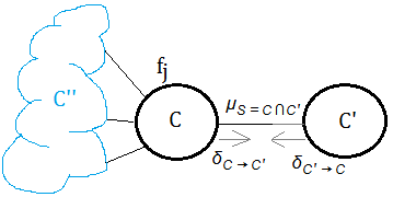
➀take $neighbor(C)$=${C”}\cup{C’}$
➁take $\mu_{S=C\cap C’}$ te be the calibrated message from clique $C$ to $C’$(or $C’$ to $C$), then
$\mu_{S=C\cap C’}$
=$\sum_{C\backslash S}\prod f_{j}\prod_{C”\in neighbor(C)}\delta_{C”\rightarrow C}$
=$\sum_{C\backslash S}\prod f_{j}\prod_{C”\in neighbor(C)\backslash C’}\delta_{C”\rightarrow C}$
$\;\;\cdot \delta_{C’\rightarrow C}$
=$\delta_{C\rightarrow C’}\cdot \delta_{C’\rightarrow C}$
, where $f_{j}$ is the function attached to clique $C$.
➂if we choose the calibrated message from clique $C$ to $C’$, then we have
$\mu_{C,C’}$
=$\delta_{C\rightarrow C’}\cdot \delta_{C’\rightarrow C}$
and, it also hods for below
$\mu_{C’,C}$
=$\delta_{C’\rightarrow C}\cdot \delta_{C\rightarrow C’}$

Before The End Of Bayesian Network Begin@20181201

[1] Brief summary

Using Bayesian network to compute probability of the query in the form of $P(X\vert E)$ is called inference, where $E$ is the observed evidence variable(s), $X$ is the query variable(s) in the network.

The Bayesian networks are useful for these tasks:
➀diagnosis of the form $P(causes\vert symptom)$, the quantitative thinking.
➁predict of the form $P(symptom\vert causes)$, the qualitative thinking.
➂classification of the form $\underset{class}{max}P(class\vert data)$.
➃decision making by given/develop certain kind of cost function in a subsystem.

I have ➀ and ➁ involved in a lot of my previous posts, in the incoming future, I expect myself to investigate ➂ and ➃, you can find some future direction in p.11~43 of A Tutorial on Inference and Learning in Bayesian Networks, Irina Rish, IBM T.J.Watson Research Center.

[2] Time to back to Reinforcement Learning

In the early May of 2018, I was struggling over reinforcement learning in exploitation versus exploration, for some terminology, prior or posterior alike, I explore to the Bayesian network, after months of exploitation, I should resume my reinforcement learning and explore to next station of unknow, maybe sooner or later involved in the Bayesian network due to this deep exploitation in these days.

Finally, the Bayesian network network is a network of multiple variables, while reinforcement learning is a network of only one variable iterating over multiple states.

Addendum

➀Graphical Models - Lecture 11: Clique Trees, Andrew McCallum, mccallum@cs.umass.edu
➁A Tutorial on Inference and Learning in Bayesian Networks, Irina Rish, IBM T.J.Watson Research Center