Lagrange Multiplier

27 Oct 2017

Why Lagrange Multiplier?

Suppose you are given a function f(x₁, x₂), and would like to find out its extreme, subject to a constraint function g(x₁, x₂) = 0;
where g(x₁, x₂) = ax₁ + bx₂ + c = d, with a, b, c, d to be any scalar, d might be 0.

The possible solution:
[1]Figure out from the constraint function g(x₁, x₂) = 0 and express x₂ in terms of x₁, like x₂ = h(x₁)
[2]Back to f(x₁, x₂) and replace x₂ with h(x₁), f(x₁, x₂) = f(x₁, h(x₁))
[3]Take partial derivative on x₁ to zero, ∂f(x₁, h(x₁)) ∕ ∂x₁ = 0, the x₁ value thus obtained would then lead us to the extreme of f(x₁, x₂)

Here comes the problem that not all objective parameters could be expressed in terms of other objective parameters in the constraint function.

The Regularized Formula for Lagrange Multiplier

We thus step further into the lagrange multiplier, usually, we will see:

ℒ(x₁, x₂, λ) = f(x₁, x₂) + λ(x₁, x₂) ... (1), where λ is the lagrange multiplier, and ℒ(x₁, x₂, λ) is the maximum likelihood function for us to come out with the λ that can optimize the extreme value of ℒ

To get the most optimal solution, ∂ℒ ∕ ∂x₁ = 0, ∂ℒ ∕ ∂x₂ = 0, ∂ℒ ∕ ∂λ = 0 must be mandatory!

Before proceed any further, we’d like to realize why (1) is the regularized formula for Lagrange Multiplier.

[1]Expand f by means of Taylor Series

➀take f(x₁, x₂,…, x_n) to be a continuous and differentiable function in Rⁿ,
➁take x = [x₁, x₂,…, x_n]^t ∈ Rⁿ,
➂then, begin from lim_x→af(x) = f(a), where x, a ∈ Rⁿ,
express lim_x→af(x) in terms of Taylor Series:
f(a) = f(x) + f′(x)(x − a) + (1 ∕ (2!))f″(x)(x − a)² + (1 ∕ (6!))f′″(x)(x − a)³ + …
f(a) ≈ f(x) + f′(x)(x − a); ignore the second derivative term,
then, f′(x) = ∂f(x) ∕ ∂x = [∂f(x) ∕ ∂x₁ ∂f(x) ∕ ∂x₂ … ∂f(x) ∕ ∂x_n]^t = ∇f,
f(a) ≈ f(x) + (∇f)^t(x − a)_n×1

[2]Next, we discuss single constraint condition

➀suppose we are asking for min/max f(x), subject to g(x) = c, cmight be 0, x ∈ Rⁿ, where g(x) = c is a continuous, differentiable hypersurface on Rⁿ
➁express lim_x→ag(x) = g(a) in terms of Taylor Series, then:
g(a) ≈ g(x) + g′(x)(x − a) = g(x) + (∇g)^t ⋅(x − a) _n×1
➂if a is also the point on the hypersurface, then, g(x) = g(a) = 0, we can treat (x − a) → 0, since x is very closed to a and conclude that (∇g)^t(x − a)_n×1 = 0
➃that is to say (∇g)^t is the normal vector orthogonal to the hypersurface at the point a, where we can have:
(∇g)^t ≈ lim_x→a[(g(x) − g(a)) ∕ (x − a)]^t
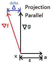
➄cautions must be made that level curve of function f might hit onto the hypersurface of function g at the point x, with an infinitesimal distance to the point a, say it ε, where x + ε = a
➅then, ∇f might not be full parallel to ∇g, we should have:
Δ = ∇f − Proj_∇g(∇f) … ≠ 0
     = ∇f − (((∇f)^t ⋅ ∇g) ∕ ||∇g||²) ⋅ ∇g
∵ε→0, x→a, we thus have Δ ≈ 0
∴Δ = ∇f − λ∇g ≈ 0, where λ = (((∇f)^t ⋅ ∇g) ∕ ||∇g||²)
or, we can directly say that ∇f ∈ span{∇g}
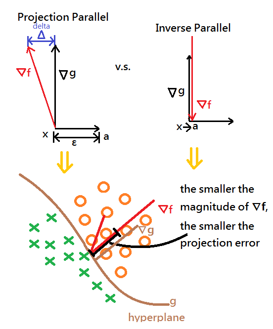
➆if your AI algorithm works well, then ε→0, such that ∇f = λ∇g could hold, we illustrate this concept of projecting ∇f onto ∇g, see below pic(the picture is just by intuition).

[3]Lagrangian representation in most application design

In most application design, Lagrange Multiplier likelihood function is expressed as:
ℒ(x, λ) = f(x) + λg(x), x ∈ Rⁿ,
∂ℒ ∕ ∂x = ∇f + λ∇g … (a)
∂ℒ ∕ ∂λ = 0 … (b)
=>Resolve above two equations (a), (b) to get λ:
➀if λ = 0, then, ∇f = 0 means that ∇f(x^*) = 0 and g(x^*) = 0 just satisfy the constraint function, where
g(x) = a₁x₁^d1 + a₂x₂^d2 + … + a_nx_n^dn + C = 0, x ∈ Rⁿ
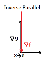
➁if λ ≠ 0, then, ∇f = -λ∇g, it implies that ∇f and ∇g are inverse parallel, where f(x) has a extreme(min/max) at this point x^*(so does g(x))
➂be noted that g(x) != 0 would not impact, since ∂ℒ ∕ ∂λ = 0 for a solve and g(x) equates to any scalar would be subject to the question domain.

[4]Why ∇f and ∇g are inverse parallel?

∵the regularization by using the lagrange multiplier would further reduce the magnitude of ∇f, the final ∇f would be normal vector with small magnitude(length), thus the small error when we project sample data onto ∇f.
This design expects a minimum magnitude of the gradient after regularization at the tangent point where the level curve and the hypersurface of the constraint function.

What to choose in between ℒ(x, λ) = f(x) + λg(x) v.s. ℒ(x, λ) = f(x) − λg(x)

It depends on exactly your design of regularization algorithm and how good you believe your regularization can work.
➀if you aims at reducing the prediction error(Δ),then, ℒ(x, λ) = f(x) − λg(x) might be the most appropriate
➁inverse parallel version of ℒ(x, λ) = f(x) + λg(x) would make the point on minimizing the magnitude of ∇f which is orthogonal to the hyperplane.
Both guarantee the projecting sample data onto ∇f would we have the minimal error(see below pic for intuition).
One thing interest is that by choosing ℒ(x, λ) = f(x) + λg(x), the λ is negative; nevertheless, ℒ(x, λ) = f(x) − λg(x) would come out with positive λ, concluded from the 2 combination, we should have the lagrgarian in a more regularized expression:
ℒ(x, λ) = f(x) + sign(λ)λg(x), where sign(λ) is negative.

The Lagrange Multiplier and Multiple Constraints

➀succeeding to conclusion in above paragraph, suppose we are asking for min/max f(x), subject to g_k(x) = 0, x ∈ Rⁿ, k = 1 to m, and g_k(x) is continuous and differentiable,
where ∇f = -∑_k=1^mλ_k∇g_k
⇔ ∇f ∈ span{∇g₁, ∇g₂,…, ∇g_m}
➁refine Lagrange Multiplier likelihood function, we have:
ℒ(x, {λ_k}) = f(x) + ∑_kλ_kg_k(x), for k = 1 to m
➂to find the extreme value(min/max), we need:
∇_xℒ = ∇f + ∑_k=1^mλ_k∇g_k = 0 … (c)
∇_λkℒ = g_k(x) = 0 for k = 1 to m … (d)