Gradient Descendent

07 Nov 2017

Gradient Descendent

Most widely used in machine learning with respect to linear regression, logistic regression for supervised learning. But, the gradient descendent itself actually knows nothing when to stop!!

Begin from Cost Function in Simple Linear Regressoin(S.L.R)

take the cost function $J(\theta)=\frac1{2m}\sum_{i=1}^m(h_\theta(x^{(i)})-y^{(i)})^2$, where the purpose of S.L.R is to minimize $J(\theta)$.
given $h_\theta(x)=\theta^t\cdot x$, where \(\theta=\begin{bmatrix}\theta_1\\\theta_2\end{bmatrix}\) is the coefficients
take \(X=\begin{bmatrix}x_1\\x_2\end{bmatrix}\) as the input data
and $x_1=1$, it is the intercept, or the bias term.
as to the divide by 2m is an artificial design:
➀$\frac12$ is to eliminate the power of 2 in the square, after differentiation is taken.
➁$\frac1m$ is to average all squared errors of m input rows of data.
➂the superscribe(i) of $X$, $Y$ are the index of the input data record, means it is the i-th input data $X$, $Y$

Step into Gradient ∇ of $J(\theta)$

suppose we are given m records of input data, they are $X$ and $Y$. ➀take derivation of $J\left(\theta \right)$ on ${\theta }_j$, then we obtain:

$\frac{\partial J\left(\theta \right)}{\partial {\theta }_j}=\frac{1}{m}\sum _{i=1}^m\left(h_{\theta }\right(x^{\left(i\right)})-y^{\left(i\right)})·x_j^{\left(i\right)}$

since we are running batch gradient descendent, $\frac{1}{m}$ is required to average it.
➁if m = 1, then, we just have the j-th term as:

$\frac{\partial J\left(\theta \right)}{\partial {\theta }_j}=\sum _{i=1}^m\left(h_{\theta }\right(x^{\left(i\right)})-y^{\left(i\right)})·x_j^{\left(i\right)}$

Learning Rate α

it is used to converge the result of gradient descendent. The smaller value would believed to have a less fluctuation.

Put It Together

put everything together, we will have the j-the term of $\theta$, it is inclusive of the bias term $\theta_1$:

${\theta }_j={\theta }_j-\alpha ·\frac{1}{m}\sum _{i=1}^m\left(h_{\theta }\right(x^{\left(i\right)})-y^{\left(i\right)})·x_j^{\left(i\right)}, where j=1 to n, \theta \in R^n$

given $X\in M_{m\times n}, \theta \in M_{n\times 1}, Y\in M_{m\times 1}, x^{\left(i\right)}\in M_{n\times 1}$,

$X={\left[\begin{array}{c}-(x^{\left(1\right)}{)}^t-\\ -(x^{\left(2\right)}{)}^t-\\ ...\\ -(x^{\left(m\right)}{)}^t-\end{array}\right]}_{mxn}$

and, we just deduce out:

$$\begin{gathered} \frac{\partial J\left(\theta \right)}{\partial {\theta }_j}=\frac{1}{m}\sum _{i=1}^m\left(h_{\theta }\right(x^{\left(i\right)})-y^{\left(i\right)})·x_j^{\left(i\right)} \\ =({\left[\begin{array}{c}-(x^{\left(1\right)}{)}^t-\\ -(x^{\left(2\right)}{)}^t-\\ ...\\ -(x^{\left(m\right)}{)}^t-\end{array}\right]}_{mxn}·{\left[\begin{array}{c}{\theta }_1\\ {\theta }_2\\ ...\\ {\theta }_n\end{array}\right]}_{n\times 1}-{\left[\begin{array}{c}{y}^{\left(1\right)}\\ y^{\left(2\right)}\\ ...\\ y^{\left(m\right)}\end{array}\right]}_{m\times 1}{)}^t·\left[\begin{array}{c}{x}_j^{\left(1\right)}\\ x_j^{\left(2\right)}\\ ...\\ x_j^{\left(m\right)}\end{array}\right]·\frac{1}{m} \end{gathered}$$

Why the Gradient Descendent Works?

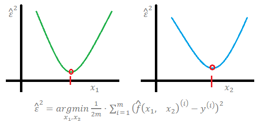
We will illustrate with cost function of multiple parameters:

➀given $f(x_1,x_2)$ a multi-parameters cost function, the gradient ∇ of $f$ are $\frac{\partial f}{\partial x_1}$, $\frac{{\displaystyle \partial f}}{{\displaystyle \partial x_2}}$
➁suppose $y=f(x_1,x_2)$
➂take ${\hat{\epsilon }}^2=\frac{1}{2m}·\sum _{i=1}^m\left(\hat{f}\right(x_1,x_2{)}^{\left(i\right)}-y^{\left(i\right)}{)}^2$
➃to get the minimum value of ${\hat{\epsilon }}^2$, we have to figure out by below function:

${\hat{\epsilon }}^2=\underset{x_1,x_2}{argmin}\frac{1}{2m}·\sum _{i=1}^m\left(\hat{f}\right(x_1,x_2{)}^{\left(i\right)}-y^{\left(i\right)}{)}^2$

, where ${\hat{\epsilon }}^2$ is a convex function
➄the gradient descendent is the algorithm that can gradually lead to final $x_1$, $x_2$ that can minimize ${\hat{\epsilon }}^2$

suppose we are beginning from some base point ${x_1}^{\left(0\right)}$, ${x_2}^{\left(0\right)}$, where the upper subscribe(0) is the iteration index, indicates that it is the 0-th iteration.

for $i$=0 to some large value.
➀${x_1}^{\left(i\right)}={x_1}^{(i-1)}-\alpha ·\frac{\partial f({x_1}^{(i-1)}, {x_2}^{(i-1)})}{\partial x_1}$
➁${x_2}^{\left(i\right)}={x_2}^{(i-1)}-\alpha ·\frac{\partial f({x_1}^{(i-1)}, {x_2}^{(i-1)})}{\partial x_2}$
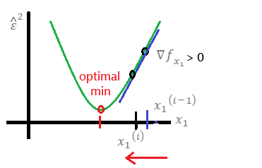
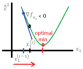
repeat above 2 steps in the same iteration, loop until the ${\hat{\epsilon }}^2$ could be believed at its minimum or the iteration index i is large enough.

next, we explain why we choose to minimize the gradient, actually, there exists 2 gradients, +∇ and −∇:
➀for +∇, the equation minus the positive gradient at learning rate α > 0, then, ${x_1}^{\left(i\right)}={x_1}^{(i-1)}-\alpha ·\nabla f_{x_1}({x_1}^{(i-1)},{x_2}^{(i-1)})$
the ${x_1}^{\left(i\right)}$ would step back to the optimal minimum.

➁for −∇, the equation minus the negative gradient at learning rate α > 0, then, ${x_1}^{\left(i\right)}={x_1}^{(i-1)}+\alpha ·\nabla f_{x_1}({x_1}^{(i-1)},{x_2}^{(i-1)})$
the ${x_1}^{\left(i\right)}$ would step forward to the optimal minimum.

both ➀, ➁ work for $x_2$ in this example, we thus prove it!!