Binary and Multiple Classification

13 Nov 2017

Classification

Classification could be categorized into two major variety, they are binary and multiple classifications. The major purpose of binary classification is to identify an object as two mutual exclusive identity by means of logistic regression. The multiple regression comes out with a wider rage of identity, might be 0, 1, 2, 3,...n, nevertheless, it is using one versus all, which is the same algorithm of binary classification.

Binary Classification

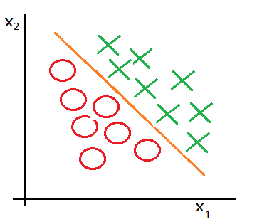
Given input data of size n, binary classification is to classify it to be true or false, or identity of another alternative, 0 and 1, and still further.
Before we step into multiple classification, a full illustration of the logistic regression model is mandatory.

Why We Need The Logistic Regression Model?

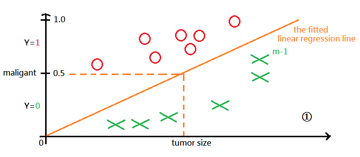
Suppose we’d like to classify the given input data as 0 or 1, in example of tumor size identification of maligant or benight.
We are given m records of tumor history and come out the fitted linear regression line in grapg labeled ➀, where m-1 th record is identified as non-maligant($Y=0$).

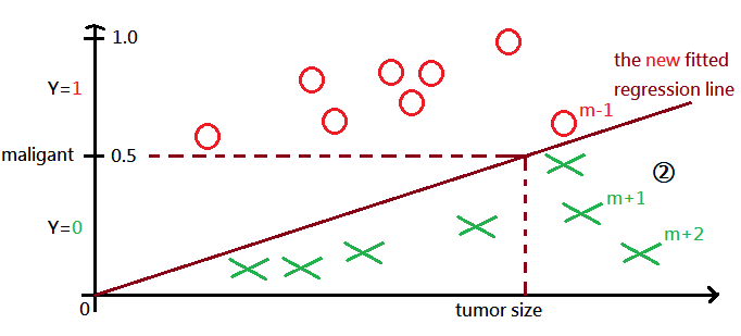
After record m+1, m+2 have been added to the given sample, we get the new fitted regression line in graph labeled ➁, watch out that m-1 th record is now identified as maligant($Y=1$)!!!

Caution must be made that by tradition, the fitted linear regression line could be biased with the input sample and $h_\theta(x)>1\;or\;<\;0$ could happen.

What we want for binary classification in this example is to classify
\(\left\{\begin{array}{l}Y=1,\;h_\theta(x)\geq0.5\\Y=0,\;h_\theta(x)<0.5\end{array}\right.\) The linear regression model is likely to have $h_\theta(x)>1\;or\;<\;0$; while the logistic regression model has $0\leq h_\theta(x)\leq1$!!!

The Logistic Regression Function

It is also named as the sigmoid function, and defined as: \(h_\theta(x)=\frac1{1+e^{-\theta^t\cdot x}},\;where\;\left\{\begin{array}{l}\theta\in R^n,\;M_{n\times1}\\x\in R^n,\;M_{n\times1}\end{array}\right.\)

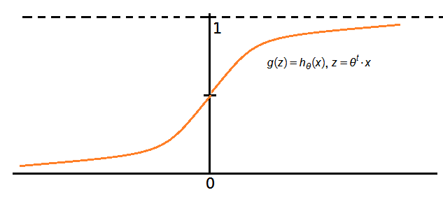
We can then have $h_\theta(x)=P(Y=1\vert x;\theta),\;the\;probablity\;of\;Y=1\;given\;x\;and\;\theta$
➀$P(Y=1\vert x;\theta)+P(Y=0\vert x;\theta)=1$
➁$P(Y=1\vert x;\theta)=1-P(Y=0\vert x;\theta)$

The Logistic Regression Cost Function

Can we re-using the cost function in linear regression model, $J(\theta)=\frac1{2m}\sum_{i=1}^m(h_\theta(x^{(i)})-y^{(i)})^2$ to be the logistic version of cost function? The answer is no!!! Because the gradient descendent wouldn’t be a smooth convex curve.

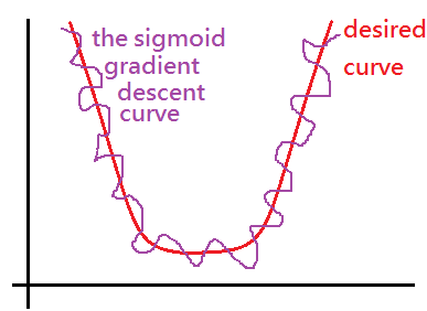
The major purpose of the cost function is to reduce the error of the model and gradient descendent could then be applied on to get the $\theta$ that can really have the smallest error.
Two key points must be clarified:
➀when $P(Y=1)\approx1$, the error from 1 for $P(Y=1)\approx0$ ➁when $P(Y=0)\approx0$, the error from 0 for $P(Y=0)\approx0$ We thus define the cost function as:
\(\left\{\begin{array}{l}-\log(h_\theta(x)),\;for\;Y=1\\-\log(1-h_\theta(x)),\;for\;Y=0\end{array}\right.\)

Why do we use log? Why to have a minus sign?

Please recall $\log1=0$, whenever $h_\theta(x)\approx1$ or $h_\theta(x)\approx0$.

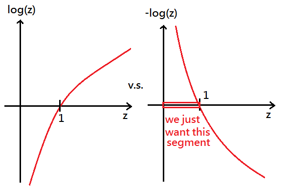
Next to formulize it,
\(\begin{array}{l}J(\theta)=\frac1m\sum_{i=1}^m\cos t(h_\theta(x^{(i)}),y^{(i)}),\\where\;\cos t(h_\theta(x^{(i)}),y^{(i)})=\left\{\begin{array}{l}-\log(h_\theta(x^{(i)})),\;for\;y^{(i)}=1\\-\log(1-h_\theta(x^{(i)})),\;for\;y^{(i)}=0\end{array}\right.\end{array}\)

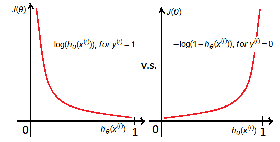
The graph exhibits some findings:
\(\left\{\begin{array}{l}\cos t(h_\theta(x^{(i)}),y^{(i)})=0,\;if\;h_\theta(x^{(i)})=y^{(i)}\\\cos t(h_\theta(x^{(i)}),y^{(i)})\approx\infty,\;if\;h_\theta(x^{(i)})\approx0,\;y^{(i)}=1\\\cos t(h_\theta(x^{(i)}),y^{(i)})\approx\infty,\;if\;h_\theta(x^{(i)})\approx1,\;y^{(i)}=0\end{array}\right.\)

Now, we combine the two cases into one formula:
\(\begin{array}{l}J(\theta)=-\frac1m\sum_{i=1}^m\lbrack y^{(i)}\cdot\log(h_\theta(x^{(i)}))+(1-y^{(i)})\cdot\log(1-h_\theta(x^{(i)}))\rbrack,\\where\;\left\{\begin{array}{l}y^{(i)}=1,\;we\;have\;1-y^{(i)}=0\\y^{(i)}=0,\;we\;have\;1-y^{(i)}=1\end{array}\right.\end{array}\) Thus, we chould have the 2 cases being operated in mutual exclusive flow.

Regularization of The Logistic Regression Cost Function

Please remind the need of regularization of cost function, or you might struggle in the overfitting embarrassed situation. We put an extra term at the end of existing cost function:
\(\begin{array}{l}\underset{REG}{J(\theta)}=-\frac1m\sum_{i=1}^m\lbrack y^{(i)}\cdot\log(h_\theta(x^{(i)}))+(1-y^{(i)})\cdot\log(1-h_\theta(x^{(i)}))\rbrack+\frac\lambda{2m}\sum_{j=1}^n\theta_j^2;\\where\;\theta\in R^n,\;M_{n\times1}\end{array}\)

For the ease of understand, we illustrate by intuition:
➀$\frac{\partial J(\theta)}{\partial\theta_j}=\frac1m\sum_{i=1}^m(h_\theta(x^{(i)})-y^{(i)})\cdot x_j^{(i)},for\;j=1,$ the bias term, no need for regularization!!!
➁$\frac{\partial J(\theta)}{\partial\theta_j}=\frac1m\sum_{i=1}^m(h_\theta(x^{(i)})-y^{(i)})\cdot x_j^{(i)}+\frac\lambda m\theta_j,\;for\;j>1$
;where the term $h_\theta(x^{(i)})-y^{(i)}$ is just the intuitive concept, the proof should make the derivation on the regularized version of cost function, next, we take the action.

Derivate the first part of cost function, we have below deduction:
\(\begin{array}{l}J(\theta)=-\frac1m\sum_{i=1}^m\lbrack y^{(i)}\cdot\log(h_\theta(x^{(i)}))+(1-y^{(i)})\cdot\log(1-h_\theta(x^{(i)}))\rbrack;\\where\;\;h_\theta(x)=\frac1{1+e^{-\theta^t\cdot x}},\;\theta\in R^n,\;x\in R^n,\\\frac{\partial J(\theta)}{\partial\theta_j}=\frac1m\sum_{i=1}^m\lbrack-y^{(i)}\cdot(h_\theta(x^{(i)}))^{-1}-(1-y^{(i)})\cdot(1-h_\theta(x^{(i)}))^{-1}\cdot\frac{\partial{(1-h_\theta(x^{(i)}))}}{\partial\theta_j}\rbrack\end{array}\)

We make further expression:
➀the first order partial differential of $h_\theta(x^{(i)})$:
\(\begin{array}{l}\frac{\partial(h_\theta(x^{(i)}))}{\partial\theta_j}\\=\frac{\partial({\displaystyle\frac1{1+e^{-\theta^t\cdot x^{(i)}}}})}{\partial\theta_j}\\=\frac{\partial(1+e^{-\theta^t\cdot x^{(i)}})^{-1}}{\partial\theta_j}\\=(-1)\cdot\lbrack1+e^{-\theta^t\cdot x^{(i)}}\rbrack^{-2}\cdot(-x_j^{(i)}\cdot e^{-\theta^t\cdot x^{(i)}})\\=\lbrack1+e^{-\theta^t\cdot x^{(i)}}\rbrack^{-2}\cdot(x_j^{(i)}\cdot e^{-\theta^t\cdot x^{(i)}})\end{array}\)

➁extend $1-h_\theta(x^{(i)})$ as:
\(1-h_\theta(x^{(i)})=1-\frac1{1+e^{-\theta^t\cdot x^{(i)}}}=\frac{e^{-\theta^t\cdot x^{(i)}}}{1+e^{-\theta^t\cdot x^{(i)}}}\)

Take ➀ and ➁ into the first order partial differential of $J(\theta)$:
\(\begin{array}{l}\frac{\partial J(\theta)}{\partial\theta_j}\\=\frac1m\sum_{i=1}^m\lbrack-y^{(i)}\cdot(1+e^{-\theta^t\cdot x^{(i)}})\cdot(1+e^{-\theta^t\cdot x^{(i)}})^{-2}\cdot(x_j^{(i)}\cdot e^{-\theta^t\cdot x^{(i)}})+\\(1-y^{(i)})\cdot(\frac{1+e^{-\theta^t\cdot x^{(i)}}}{e^{-\theta^t\cdot x^{(i)}}})\cdot(1+e^{-\theta^t\cdot x^{(i)}})^{-2}\cdot(x_j^{(i)}\cdot e^{-\theta^t\cdot x^{(i)}})\rbrack\\=\frac1m\sum_{i=1}^m\lbrack-y^{(i)}\cdot(1+e^{-\theta^t\cdot x^{(i)}})^{-1}\cdot(x_j^{(i)}\cdot e^{-\theta^t\cdot x^{(i)}})+\\(1-y^{(i)})\cdot e^{\theta^t\cdot x^{(i)}}\cdot(1+e^{-\theta^t\cdot x^{(i)}})^{-1}\cdot(x_j^{(i)}\cdot e^{-\theta^t\cdot x^{(i)}})\rbrack\\=\frac1m\sum_{i=1}^m\lbrack-y^{(i)}\cdot(1+e^{-\theta^t\cdot x^{(i)}})^{-1}\cdot(e^{-\theta^t\cdot x^{(i)}}\cdot x_j^{(i)})+\\(1-y^{(i)})\cdot(1+e^{-\theta^t\cdot x^{(i)}})^{-1}\cdot x_j^{(i)})\rbrack\\=\frac1m\sum_{i=1}^m\lbrack-y^{(i)}\cdot(e^{-\theta^t\cdot x^{(i)}}\cdot x_j^{(i)})+(1-y^{(i)})\cdot x_j^{(i)})\rbrack\cdot(1+e^{-\theta^t\cdot x^{(i)}})^{-1}\\=\frac1m\sum_{i=1}^m\lbrack-y^{(i)}\cdot(e^{-\theta^t\cdot x^{(i)}}\cdot x_j^{(i)})+(1-y^{(i)})\cdot x_j^{(i)})\rbrack\cdot h_\theta(x^{(i)})\end{array}\)

Finally, take the second part together in the derivative, we get the total solution:
\(\frac{\partial J(\theta)_{REG}}{\partial\theta}=\frac{\displaystyle1}{\displaystyle m}\sum_{i=1}^m\lbrack-x^{(i)}\cdot y^{(i)}\cdot e^{-\theta^t\cdot x^{(i)}}+x^{(i)}\cdot(1-y^{(i)})\rbrack\cdot h_\theta(x^{(i)})+\frac\lambda m\theta\)

Multiple Classification

We now migrate to multiple classification. There might exist more than one pattern in the given sampling, how do you plan to classify the object to the correct identity? We introduce the most often used method, one-versus-all.
Take $h_\theta^{(k)}(x^{(i)})=P(y^{(i)}=k\vert\theta^{(k)},x^{(i)});\;k=1,2,3,\;i=1\;to\;m,\;the\;count\;of\;data\;set$. Next to illustrate one-versus-all method:

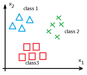
➀train with $h_\theta^{(1)}(x^{(i)})$ to get the desired $\theta^{(1)}$ vector for class 1.

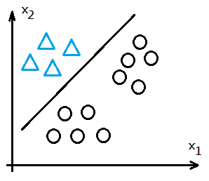
➁train with $h_\theta^{(2)}(x^{(i)})$ to get the desired $\theta^{(2)}$ vector for class 2.

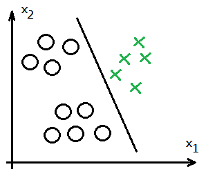
➂train with $h_\theta^{(3)}(x^{(i)})$ to get the desired $\theta^{(3)}$ vector for class 3.

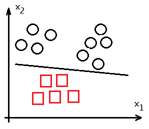
After $\theta^{(k)}$ has been figured out, for any new input of $x^{(i)}$, where $i\geq m$, use $h_\theta^{(k)}(x^{(i)})$ to predict the output, and choose the maximum one as the object identity.

That is to say $\underset k{max}\;h_\theta^{(k)}(x^{(i)})$ as the identity of class k.