Introduction To The Exponential Distribution

24 Jan 2018

Prologue To The Exponential Distribution

In probability theory and statistics, the exponential distribution is the model of distribution further developed, base on the most fundamental gamma distribution. With the basic realization of gamma distributions, we could also treat the exponential distribution a special case of gamma distribution. It would be greatly helpful in the evaluation of the experimental model build on your hypothesis, the power of test for the precision in the machine learning results.

The Exponential Distribution Illustration

This article would like to guide you through a design of a simple case to generalize the exponential distribution.

➀the experiment is proceeded with the assumption that $x$ is the rate of event occurrence during one time interval $t$, totally, $x\cdot t$ events.
➁suppose $V$ is the volumetric space where these events occur within. Trivially, the success probability of event occurrence, we take it as $P_{success}$=$\frac {x\cdot t}{V}$, then the failure probability could be regarded as $P_{fail}$=$1-\frac {x\cdot t}{V}$.
➂suppose the rate $x$ do exist and remain constant over each disjoint interval for some event occurrence.
➃each disjoint interval are of the same time length, say it $t$, and we further divide it into n subsections. Then each subsection would have $P_{success}$=$\frac {x\cdot t}{V\cdot n}$, then the failure probability could be regarded as $P_{fail}$=$1-\frac {x\cdot t}{V\cdot n}$.
➄we assume that each occurrence of the event in distinct subsection is independent, the success v.s. failure probability in each subsection just matches the the Bernoulli distribution.
➅let the random variable $T$ to be the time it takes until the very first event to occur, and the whole behavior follows the geometric distribution, if it takes time larger than time $t$ for the very first event to occur, then we have such probability:
$P(T>t)$=$\lim_{n\rightarrow\infty}(P_{fail})^{n}$=$\lim_{n\rightarrow\infty}(1-\frac {x\cdot t}{V\cdot n})^{n}$

$(1-\frac {x\cdot t}{V\cdot n})^{n}$
$=C_{0}^{n}1^{n}\cdot(-\frac {x\cdot t}{V\cdot n})^{0}$+$C_{1}^{n}1^{n-1}\cdot(-\frac {x\cdot t}{V\cdot n})^{1}$+$C_{2}^{n}1^{n-2}\cdot(-\frac {x\cdot t}{V\cdot n})^{2}$+…+$C_{n}^{n}1^{0}\cdot(-\frac {x\cdot t}{V\cdot n})^{n}$

Since $\lim_{n\rightarrow\infty}(-\frac {x\cdot t}{V\cdot n})=0$, then:
$P(T>t)$
$=\lim_{n\rightarrow\infty}(1-\frac {x\cdot t}{V\cdot n})^{n}$
$=\lim_{n\rightarrow\infty}1+(-\frac {x\cdot t}{V\cdot n})^{n}$
$\approx\lim_{n\rightarrow\infty}(1+\frac {-x\cdot t}{V\cdot n})^{n}$

Since $e$=$\lim_{n\rightarrow\infty}(1+\frac {1}{n})^{n}$, and
$e^{2}$=$\lim_{n\rightarrow\infty}((1+\frac {1}{n})^{n})^{2}$
$=\lim_{n\rightarrow\infty}((1+\frac {1}{n})^{2})^{n}$
$=\lim_{n\rightarrow\infty}(1+\frac {2}{n}+\frac {1}{n^{2}})^{n}$
$\approx\lim_{n\rightarrow\infty}(1+\frac {2}{n})^{n}$

Then, $P(T>t)$=$e^{-\frac {x\cdot t}{V}}$

➆therefore, $P(T\le t)$=$1-e^{-\frac {x\cdot t}{V}}$, it is the successful probability for events to occur within time $t$.

Above is just the basic illustration of the the exponential distribution. Such scenario would be mostly found in chemical catalyst experiment, or fermentation test in biological laboratory.

Definition Of The Exponential Distribution

Succeeding to the last paragraph, for the simplicity, we take $\lambda$=$\frac {x}{V}$ to be the rate, the intensity. The CDF could be easily defined as below:
$F_{T}(t)$=$1-e^{-\lambda\cdot t}$=$P(T\le t)$

Derivate $F_{T}(t)$ on $t$, we then get its PDF below:
$f_{T}(t)$=$\frac{\operatorname d{F_{T}(t)}}{\operatorname d{t}}$=$\lambda\cdot e^{-\lambda\cdot t}$

To validate it,
$P(T\le a)$
$=\int_{0}^{a}\lambda\cdot e^{-\lambda\cdot t}\operatorname dt$
$=-e^{-\lambda\cdot t}\vert_{0}^{a}$
$=1-e^{-\lambda\cdot a}$, take $t$=$a$

Relationship With The Gamma Distribution

Be recalled that the PDF of the gamma distribution:
$f_{X}(x)=\frac {1}{\beta^{\alpha}\cdot\Gamma(\alpha)}\cdot x^{\alpha-1}\cdot e^{-\frac{x}{\beta}}$

Take $\alpha$=$1$, $\lambda$=$\frac {1}{\beta}$, you can easily find that the exponential distribution a special case of gamma distribution. Change $X$ to $T$, $x$ to $t$, they are exactly the same thing!!!

Below chart exhibits its PDF with regards to $\lambda$ set to $0.5$,$0.333$:
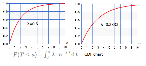
Next chart illustrate the cumulative distribution with $\lambda$ set to $0.5$,$0.333$:

Moments Of The Exponential Distribution

The most efficient way to get the expect value and variance would be the moments.
➀take $\alpha$=$1$, $\lambda$=$\frac {1}{\beta}$, we will have the moments below:
$\mu_{r}$=$E\lbrack X^{r}\rbrack$=$\frac {1}{\beta}\int_{0}^{\infty}x^{r}\cdot e^{-\frac {x}{\beta}}\operatorname dx$

➁let $y$=$\frac {x}{\beta}$, $\operatorname dy$=$\frac {1}{\beta}\cdot\operatorname dx$, then:
$\mu_{r}$=$\frac {1}{\beta}\int_{0}^{\infty}(\beta\cdot y)^{r}\cdot e^{-y}\cdot\beta\cdot\operatorname dy$
$\;\;\;\;$=$\beta^{r}\int_{0}^{\infty}(y)^{r}\cdot e^{-y}\operatorname dy$
$\;\;\;\;$=$\beta^{r}\cdot\Gamma(r+1)$

Therefore, we have $\mu_1$=$\beta\cdot\Gamma(2)$=$\beta$
And $\mu_2$=$\beta^{2}\cdot\Gamma(3)$=$\beta^{2}\cdot 2\cdot\Gamma(2)$=$2\cdot\beta^{2}$

Finally, the expect value $\mu_{1}$=$E\lbrack X\rbrack$=$\beta$
The variance $Var\lbrack X\rbrack$=$E\lbrack X^2\rbrack$-$E^2\lbrack X\rbrack$=$\beta^{2}$
Recall that we take $\lambda$=$\frac {1}{\beta}$, hence, $E\lbrack X\rbrack$=$\frac {1}{\lambda}$, $Var\lbrack X\rbrack$=$(\frac {1}{\lambda})^2$