Introduction To The Poisson Process Inter-arrival Times
23 Apr 2018Prologue To The Poisson Process Inter-arrival Times
The Inter-arrival Times
Given that $X_{1}$,$X_{2}$,…,$X_{n}$ are random variables with event outcome occurrences arrived at specific time. To make it more formally, we take the difference $T_{i}$=$X_{i}$-$X_{i-1}$ as the inter-arrival times.
The Very First Inter-arrival Times Follows Exponential Distribution
We start to derive the probability distribution of inter-arrival times, let’s focus on the very first one as the prelude.
$P(T_{1}\le t)$
➀take $T_{1}$=$X_{1}$ as the very first arrival time.
➁the probability of first arrival at time greater than t is equivalent to the probability of zero arrival within time $[0,t]$.=1-$P(T_{1}>t)$=1-$P(N_{[0,t]}=0)$=1-$e^{-\lambda\cdot t}$
The very first inter-arrival times is itself an exponential distribution.
, where $\lambda$ is the intensity, the rate of event occurrence.
The Distribution Of Distinct Inter-arrival Times
If you take a close look at the random arrivals over the horizon, trivially, numerous distinct inter-arrival times could be found.
Suppose you are given two adjacent inter-arrival times, $T_{i}$=$s$,$T_{i+1}$=$t$. We are asking the probability for we have the second arrival after time duration $t$, under the condition that we have the first arrival with regards to $T_{i}$=$s$.
This turns into the conditional probability.
$P(T_{i+1}>t|T_{i}=s)$
=$P(T_{i+1}>t,T_{i}=s|T_{i}=s)$
=$P(N_{(s,s+t]}=0,N_{[0,s]}=1|N_{[0,s]}=1)$
=$\frac {P(N_{(s,s+t]}=0\cap N_{[0,s]}=1)}{P(N_{[0,s]}=1)}$
=$\frac {P(N_{(s,s+t]}=0)\cdot P(N_{[0,s]}=1)}{P(N_{[0,s]}=1)}$…independence
=$P(N_{(s,s+t]}=0)$
=$e^{-\lambda\cdot(t)}$Therefore, $P(T_{i+1}\le t|T_{i}=s)$=1-$P(T_{i+1}>t|T_{i}=s)$=1-$e^{-\lambda\cdot(t)}$
We can claim that each distinct inter-arrival times has an exponential distribution. Some textbook treat it as the one-dimensional Poisson process.
The Joint Distribution Of Random Arrivals::mjtsai1974
Due to the nature of the exponential distribution, we can then derive the joint distribution of numerous random arrivals in the unit of each distinct inter-arrival times as a whole.
proof::mjtsai1974
By one-dimensional Poisson process, we know that all $T_{i}$’s are independent and each has an $Exp(\lambda\cdot t)$ distribution, where $t$ is the inter-arrival times. Let me state below claim:
➀$T_{i}$=$X_{i}$-$X_{i-1}$
➁$X_{i}$=$T_{i}$+$T_{i-1}$
➂where ➀,➁is the rule for each new arrival, $T_{0}$=$X_{0}$=$0$ by default.
Then, $F_{T_{i}}$=$P(T_{i}\le t)$=1-$e^{-\lambda\cdot t}$, for $i$=$1$,$2$,$3$,…
I’d like to prove that the joint distribution of random arrivals is just a gamma distribution.
[1]begin by time tick at $0$, say we use $X_{1}$ as the random variable to represent the first one arrival within whatever time length $t$ is, denote time period $[0,t]$ as $T_{1}$.
➀$F_{X_{1}}(t)$=$F_{T_{1}+T_{0}}(t)$=$P(T_{1}\le t)$=1-$e^{-\lambda\cdot t}$, where $T_{0}$=$0$
➁$f_{X_{1}}(t)$=$\lambda\cdot e^{-\lambda\cdot t}$
Trivially, by previous section, each $X_{i}$ just has an exponential distribution.
[2]for whatever $T_{1}$ is, after that, say we’d like to have the second arrival within time length $t$, and use the $X_{2}$ as the random variable for the second arrival.
➀$T_{2}$=$X_{2}$-$X_{1}$ and $X_{2}$=$T_{2}$+$T_{1}$
➁$F_{X_{2}}(t)$
=$F_{T_{2}+T_{1}}(t)$
=$P(T_{2}+T_{1}\le t)$…take $Y$=$T_{1}$,$X$=$T_{2}$
=$\int_{0}^{t}\int_{0}^{t-y}f_{X}(x)\cdot f_{Y}(y)\operatorname dx\operatorname dy$
=$\int_{0}^{t}F_{X}(t-y)\cdot f_{Y}(y)\operatorname dy$
➂differentiate $F_{X_{2}}(t)$ with respect to its current variable, say $t$.
$f_{X_{2}}(t)$
=$\int_{0}^{t}f_{X}(t-y)\cdot f_{Y}(y)\operatorname dy$
=$\int_{0}^{t}\lambda\cdot e^{-\lambda\cdot(t-y)}\cdot\lambda\cdot e^{-\lambda\cdot y}\operatorname dy$
=$\lambda^{2}\cdot e^{-\lambda\cdot t}\int_{0}^{t}\operatorname dy$
=$\lambda^{2}\cdot t\cdot e^{-\lambda\cdot t}$If you set $X$=$T_{1}$,$Y$=$T_{2}$ in deduction, still the same result you can get.
[3]for whatever $T_{2}$ is, after that, we use the $X_{3}$ as the random variable for the third arrival, and would like to have it within time length $t$.
➀$X_{3}$=$T_{3}$+$T_{2}$+$T_{1}$
➁$F_{X_{3}}(t)$
=$F_{T_{3}+T_{2}+T_{1}}(t)$
=$P(T_{3}+T_{2}+T_{1}\le t)$…take $Y$=$T_{2}$+$T_{1}$,$X$=$T_{3}$
=$\int_{0}^{t}\int_{0}^{t-y}f_{X}(x)\cdot f_{Y}(y)\operatorname dx\operatorname dy$
=$\int_{0}^{t}F_{X}(t-y)\cdot f_{Y}(y)\operatorname dy$
➂differentiate $F_{X_{3}}(t)$ with respect to its current variable, say $t$.
$f_{X_{3}}(t)$
=$\int_{0}^{t}f_{X}(t-y)\cdot f_{Y}(y)\operatorname dy$
=$\int_{0}^{t}\lambda\cdot e^{-\lambda\cdot(t-y)}\cdot(\lambda)^{2}\cdot y\cdot e^{-\lambda\cdot y}\operatorname dy$
=$\lambda^{3}\cdot e^{-\lambda\cdot t}\int_{0}^{t}y\operatorname dy$
=$\frac {1}{2}\cdot\lambda^{3}\cdot t^{2}\cdot e^{-\lambda\cdot t}$If you set $X$=$T_{2}$+$T_{1}$,$Y$=$T_{3}$ in deduction, still the same result you can get.
[4]repeat above procedure until $n\rightarrow\infty$, we will have $F_{X_{n}}(t)$ holds to have its derivative $f_{X_{n}}(t)$=$\frac {\lambda\cdot(\lambda\cdot t)^{n-1}\cdot e^{-\lambda\cdot t}}{(n-1)!}$, for $n$=$1$,$2$,…, where $\Gamma(n)$=$(n-1)!$.
[5]by means of mathematics induction, we can conclude that the joint distribution of random arrivals is just a gamma distribution. Be recalled that $f_{X_{n}}(t)$=$\frac {\lambda\cdot(\lambda\cdot t)^{n-1}\cdot e^{-\lambda\cdot t}}{(n-1)!}$ is a gamma probability function in Introduction To The Gamma Distribution.
Example: Illustrate The Poisson Probability For Points Distribution
Suppose you are given $n$ points randomly generated within an interval, how to evaluate the points location? Just treat the inter-arrival times as the location info, it suffice to evaluate the probability of points arrival by means of Poisson distribution.
Let’s say the interval is $[0,a]$, explore one arrival case within this interval as a beginning.
$P(X_{1}\le s|N_{[0,a]}=1)$
[1]assume $0<s<a$, we now know one arrival occurred within $[0,a]$, the probability of this one arrival occurrence within $s$, under the condition that this occurrence is within $[0,a]$:=$P(X_{1}\le s,N_{[0,a]}=1|N_{[0,a]}=1)$
$X_{1}$ is uniformly distributed within $[0,a]$
=$P(N_{(0,s]}=1,N_{[0,a]}=1|N_{[0,a]}=1)$
=$P(N_{(0,s]}=1,N_{[s,a]}=0|N_{[0,a]}=1)$
=$\frac {\lambda\cdot s\cdot e^{-\lambda\cdot s}\cdot e^{-\lambda\cdot(a-s)}}{\lambda\cdot a\cdot e^{-\lambda\cdot a}}$
=$\frac {s}{a}$, given the event ${N_{[0,a]}=1}$ as the condition, since $\sum_{i=1}^{s}\frac {1}{a}$=$\frac {s}{a}$.
proof::mjtsai1974
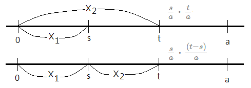
[2]suppose that there are two arrivals in $[0,a]$, that is $N_{[0,a]}=2$, and given $0<s<t<a$, we can show $P(X_{1}\le s,X_{2}\le t|N_{[0,a]}=2)$=$\frac {t^{2}-(t-s)^{2}}{a^{2}}$.➀this is to ask out the probability that first arrival falls within $[0,s]$, the second arrival falls within $(s,t]$. Below graph exhibits the possible cases.
➁by above table, we just need to accumulate the probability of the case (1) and (2), which is equivalent to substract the probability of two event occurrences in $(s,t]$ from the probability that two event arrivals in $[0,t]$.
$P(X_{1}\le s,X_{2}\le t|N_{[0,a]}=2)$
=$\frac {P(X_{1}\le s,X_{2}\le t\cap N_{[0,a]}=2)}{P(N_{[0,a]}=2)}$
=$\frac {P(X_{1},X_{2}\le t)-P(s<X_{1},X_{2}\le t)}{P(N_{[0,a]}=2)}$
=$\frac {P(N_{[0,t]}=2)\cdot P(N_{(t,a]}=0)-P(N_{[0,s)}=0)\cdot P(N_{[s,t]}=2)\cdot P(N_{(t,a]}=0)}{P(N_{[0,a]}=2)}$
=$\frac {\frac {(\lambda\cdot t)^{2}}{2!}\cdot e^{-\lambda\cdot t}\cdot\frac {(\lambda\cdot(a-t))^{0}}{0!}\cdot e^{-\lambda\cdot(a-t)}-\frac {(\lambda\cdot s)^{0}}{0!}\cdot e^{-\lambda\cdot s}\cdot\frac {(\lambda\cdot(t-s))^{2}}{2!}\cdot e^{-\lambda\cdot(t-s)}\cdot\frac {(\lambda\cdot(a-t))^{0}}{0!}\cdot e^{-\lambda\cdot(a-t)}}{\frac {(\lambda\cdot a)^{2}}{2!}\cdot e^{-\lambda\cdot a}}$
=$\frac {\frac {(\lambda\cdot t)^{2}}{2!}\cdot e^{-\lambda\cdot t}-\frac {(\lambda\cdot(t-s))^{2}}{2!}\cdot e^{-\lambda\cdot(t-s)-\lambda\cdot s-\lambda\cdot(a-t)}}{\frac {(\lambda\cdot a)^{2}}{2!}\cdot e^{-\lambda\cdot a}}$
=$\frac {\frac {(\lambda\cdot t)^{2}}{2!}\cdot e^{-\lambda\cdot t}-\frac {(\lambda\cdot(t-s))^{2}}{2!}\cdot e^{-\lambda\cdot a}}{\frac {(\lambda\cdot a)^{2}}{2!}\cdot e^{-\lambda\cdot a}}$
=$\frac {t^{2}-(t-s)^{2}}{a^{2}}$Cautions must be made that the event order just matters.
$X_{1}$,$X_{2}$ are uniformly distributed within $[0,a]$
➂$P(X_{1}\le s,X_{2}\le t|N_{[0,a]}=2)$
=$\frac {t^{2}-(t-s)^{2}}{a^{2}}$
=$\frac {t-(t-s)}{a}\cdot\frac {t+(t-s)}{a}$
=$\frac {s}{a}\cdot\frac {t+(t-s)}{a}$
=$\frac {s}{a}\cdot\frac {t}{a}$+$\frac {s}{a}\cdot\frac {(t-s)}{a}$
, given the event ${N_{[0,a]}=2}$ as the condition.
Therefore, we can claim that the Poisson process has $n$ random arrivals in time inteerval $[a,b]$, the locations of these points are independent distributed, and each of them has a uniform distribution.

