Introduction To The Probability
25 May 2018Prologue To Introduction To The Probability
Begin From The Fundamental
[1] sample space➀sample space is just the set of elements describing the outcomes of the test, experiment, formally, the result after execution of certain action.
[2] event
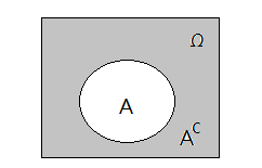
In statistics reference text book, the letter $\Omega$ is most often used to represent the sample space.
➁by flipping a coin one time, you will have two outcomes of head and tail, that is to say we associate the sample space with the set $\Omega$=$\{H,T\}$.
➂to guess the birthday within one week, the sample space $\Omega$=$\{Sun,Mon,Tue,Wed,Thu,Fri,Sat\}$.➀subset of a sample space is treated as event.
[3] intersection, union, complement
➁in the birthday in one week example, suppose we’d like to ask for the days with uppercase “S” as the prefix, then, we can denote $S$=$\{Sun,Sat\}$.
➂suppose we’d like to ask for the days with uppercase “T” as the prefix, then, we can denote $T$=$\{Tue,Thu\}$.Suppose $A$ and $B$ are two events in the sample space $\Omega$.
[4] disjoint events
➀intersection, it’s an event operator, denoted by $\cap$.
➁union, also an event operator, denoted by $\cup$.
➁complement, an event operator, usually denoted by lowercase $c$.
Suppose $A$ and $B$ are two events in the sample space $\Omega$. They are said to be two disjoint events if they have no intersection. $A\cap B$=$0$.
Such events might be regarded as mutually exclusive.
The Probability
[1] why do we need the probability?In order to express how likely it is that an event will occur, during the experiment, by assigning probability to each distinct event would be common. To distribute the probability accurately would not be an easy task.
[2] the probability functionSince each event would be associated with a probability, then we are in need of the probability function.
[3] the probability is defined on events, not on outcomes
➀the uppercase “P” is the probability function on a sample space $\Omega$ to assign the event $A$ in $\Omega$ a number $P(A)$ in $[0,1]$. The number $P(A)$ is the probability of the occurrence of event $A$.
➁wherein $P(\Omega)$=$1$
➂$P(A\cup B)$=$P(A)$+$P(B)$-$P(A\cap B)$, where $P(A\cap B)$=$0$ for $A$ and $B$ are disjoint. If $A$,$B$,$C$ are disjoint events, then $P(A\cup B\cup C)$=$P(A)$+$P(B)$+$P(C)$.➀tossing a coin one time would we have $\Omega$=$\{H,T\}$, then $P(\{H\})$=$\frac {1}{2}$, $P(\{T\})$=$\frac {1}{2}$, under the assumption that head and tail chances are coming to an equilibrium.
[4] additivity of probability
➁given cards of read, blue, green colours. The permutation of all the possible orders of cards would be $\Omega$=$\{RGB$,$RBG$,$GRB$,$GBR$,$BRG$,$BGR\}$.
$P(\{RGB\})$=$P(\{RBG\})$=$P(\{GRB\})$=$P(\{GBR\})$=$P(\{BRG\})$=$P(\{BGR\})$=$\frac {1}{6}$…the same probability for each distinct event.
➂the same example as above, the probability of the event that green card is in the middle would be $P(\{RGB,BGR\})$=$\frac {1}{3}$.
The $\{RGB,BGR\}$ is such event we desire, wherein the $\{RGB\}$ and $\{BGR\}$ are the outcomes described by $\Omega$.➀using the same card example, the probability of the event that green card is in the middle could be $P(\{XGX\})$=$P(\{RGB\})$+$P(\{BGR\})$=$\frac {1}{3}$.
This implies that the probability of an event could be obtained by summing over the probabilities of the outcomes belonging to the same event.
➁given $A$ is an event, then $P(A)$+$P(A^{c})$=$P(\Omega)$=$1$.
➂if $A$, $B$ are not disjoint, then $A$=$(A\cap B)\cup(A\cap B^{c})$, this is a disjoint union.
Therefore, $P(A)$=$P(A\cap B)$+$P(A\cap B^{c})$.
Product Of Sample Space
[1] run the same test over multiple timesTo justify the experiment result, one single test would be executed over multiple times.
[2] combine the sample space from different tests
➀suppose we flip the same coin over 2 times, the sample space $\Omega$=$\{H,T\}$x$\{H,T\}$.
It is now $\Omega$=$\{HH,HT,TH,TT\}$. Total 4 outcomes in it, we can take one outcome as one event, then $P(\{HH\})$=$P(\{HT\})$=$P(\{TH\})$=$P(\{TT\})$=$\frac {1}{4}$, under the assumption that $P(\{H\})$=$P(\{T\})$ in each single tossing of coin.➀given that 2 sample spaces with respect to 2 different tests’ outcomes, they are $\Omega_{1}$,$\Omega_{2}$, where sizeof($\Omega_{1}$)=$r$, sizeof($\Omega_{2}$)=$s$.
[3] general form of the same test over multiple times
➁then $\Omega$=$\Omega_{1}$x$\Omega_{2}$, sizeof($\Omega$)=$r\cdot s$. If we treat each distinct combination in the sample space as one single event, the probability of such distinct event is $\frac {1}{r\cdot s}$. The $\frac {1}{r}$,$\frac {1}{s}$ are the probability for the occurrences of outcomes in the $\Omega_{1}$ and $\Omega_{2}$ with respect to test 1 and test 2.➀suppose we’d like to make the experiment for n runs. We take $\Omega_{i}$ to be the sample space of the i-th test result, $\omega_{i}$ to be one of the outcomes in $\Omega_{i}$.
➁if the occurrence of each outcome $\omega_{i}$ has probability $p_{i}$, then $P(\{\omega_{1},\omega_{2}…\omega_{n}\})$=$p_{1}\cdot p_{2}…p_{n}$, which is the probability for the event $\{\omega_{1},\omega_{2}…\omega_{n}\}$ to take place.
➂assume we flip a coin with probability $p$ of head, that implies $1-p$ of tail. Then the probability of 1 single head after 4 times of tossing would be $4\cdot (1-p)^3\cdot p$.
The sample space would be
$\Omega$=$\{(HTTT),(THTT),(TTHT),(TTTH)\}$. There are 4 combinations, with each has probability $(1-p)^{3}\cdot p$.
An Infinite Sample Space
[1] run the same test until succeeds➀suppose we’d like to toss a coin until it appears with head. If the tail is always the result, the sample space $\Omega$=$\{T_{1},T_{2},T_{3},…,T_{n}…\}$, $n\rightarrow\infty$.
[2] run the same test until succeeds
Next to ask the probability function of this sample space. Assume the probability of head is $p$, the tail is $1-p$.➀for the simplicity, we’d like to change the notation by $\Omega$=$\{1,2,..,n,…\}$ for the number of iterations the tossing coin result coming out with a head.
➁$P(1)$=$P(\{H\})$=$p$
➂$P(2)$=$P(\{TH\})$=$(1-p)\cdot p$
➃$P(n)$=$P(\{T_{1}T_{2}…T_{n-1}H_{n}\})$=$(1-p)^{n-1}\cdot p$
➄when $a$ is incredibly large, the total probability becomes
$\lim_{n\rightarrow\infty}P(1)+P(2)+…+P(n)$
=$\lim_{n\rightarrow\infty}p+(1-p)\cdot p+…+(1-p)^{n-1}\cdot p$
=$\lim_{n\rightarrow\infty}p\cdot\frac {1}{1-(1-p)}$
=$p\cdot\frac {1}{p}$
=$1$…the total probabilityIn an infinite sample space, if all the events $A_{1}$,$A_{2}$,…,$A_{n}$ are disjoint, then,
$P(\Omega)$
=$P(A_{1}\cup A_{2}\cup…\cup A_{n})$
=$P(A_{1})$+$P(A_{2})$+…$P(A_{n})$
=$1$
