Propagation In The Bayesian Network
26 Aug 2018Prologue To Propagation In The Bayesian Network
Posterior Probability(Belief) Update Upon New Evidence Arrives
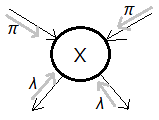
[1] Posterior probability(belief)The posterior probability(belief) of a random variable $X$=$x$, given evidence $E$=$e$, is expressed as $Bel(x)\overset\triangle=P(x\vert e)$. The evidence could be further classified as 2 distinct subsets:
[2] Deduction of $Bel(x)$
➀$e_{X}^{-}$ denotes the evidence introduced through its children nodes.
➁$e_{X}^{+}$ stands for the evidence coming from its parent nodes, for $X$ to be a root node, $e_{X}^{+}$ is the background.Assume $e_{X}^{-}$ and $e_{X}^{+}$ are independent, then the belief of $X$=$x$:
$Bel(x)$
=$P(x\vert e_{X}^{-},e_{X}^{+})$
=$\frac {P(e_{X}^{-},x\vert e_{X}^{+})}{P(e_{X}^{-}\vert e_{X}^{+})}$
=$\frac {P(e_{X}^{-}\vert x,e_{X}^{+})\cdot P(x\vert e_{X}^{+})}{P(e_{X}^{-}\vert e_{X}^{+})}$
=$\frac {P(e_{X}^{-}\vert x)\cdot P(x\vert e_{X}^{+})}{P(e_{X}^{-})}$Why we have such deduction?
[3] Generalization of $Bel(x)$
➀the evidence $e_{X}^{-}$ is given by hypothesis $X$=$x$, and the background context $e_{X}^{+}$, that explains $P(e_{X}^{-}\vert x,e_{X}^{+})$.
➁$P(x\vert e_{X}^{+})$ says that the hypothesis $X$=$x$ is propagated from the background context $e_{X}^{+}$.
➂the normalizing factor $P(e_{X}^{-}\vert e_{X}^{+})$ encompasses everything ranging from the background context to the final observed evidence, since $e_{X}^{-}$ and $e_{X}^{+}$ are independent, the denominator part becomes $P(e_{X}^{-})$.
$P(e_{X}^{-})$
=$P(e_{X}^{-}\vert e_{X}^{+})$
=$P(e_{X}^{-}\vert x,e_{X}^{+})\cdot P(x\vert e_{X}^{+})$
=$P(e_{X}^{-}\vert x)\cdot P(x\vert e_{X}^{+})$
=$\lambda(X)\cdot\pi(X)$Most of the textbooks have below common definition:
➀$\pi(x)$=$P(x\vert e_{X}^{+})$ is the respective(predictive) direction of propagation.
➁$\lambda(x)$=$P(e_{X}^{-}\vert x)$ is retrospective(diagnostic) direction of propagation.We thus express the belief of $x$ as $Bel(x)$=$\alpha\cdot\pi(x)\cdot\lambda(x)$,
[4] Message passing is propagation
where $\alpha$ is the normalizing constant, in this illustration,
$\alpha$
=$[P(e_{X}^{-})]^{-1}$
=$[\sum_{x}\pi(x)\cdot\lambda(x)]^{-1}$
New evidence enters a network when a variable is instantiated, ie when it receives a new value from the outside world. When this happens, the posterior probability of each node in the whole network must be re-calculated.
This is achieved by message passing, known as progapation.
Propagation Illustration In Causal Tree
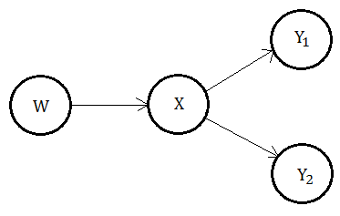
Given a causal tree of this serial chain Bayesian network, where $\lambda(Y)$=$P(e_{Y}^{-}\vert Y)$.
[1] Forward propagation
➀$W$ is now the root node, the background context is the only forward propagated evidence.
Node $X$ receives $W$ forward propagated evidence $P(w\vert e_{W}^{+})$, with each $X=x$ weighted by $P(x\vert w)$ for all $w\in W$.
$\pi(w)$=$P(w\vert e_{W}^{+})$=$P(w)$, for $w\in W$.
➁for node $X$, it receives the forward propagated evidence pass through it, thus:
$\pi(x)$
=$P(x\vert e_{X}^{+})$
=$P(x\vert e_{WX}^{+})$
=$\sum_{w}P(x\vert w)\cdot P(w\vert e_{W}^{+})$, for $w\in W$.
$\Rightarrow\pi(X)$=$P(X\vert W)\cdot\pi(W)$➂similarly, $\pi(Y)$=$P(Y\vert X)\cdot\pi(X)$
[2] Backward propagation➀$Y$ is the leaf node, the evidence of observation is the only backward propagated message.
For each $x\in X$, $\lambda(x)$ is weighted by $P(y\vert x)$ with $\lambda(y)$, for all $y\in Y$.
$\lambda(y)$=$P(e_{Y}^{-}\vert y)$
➁as $X$ receives the backward propagated evidence from $Y$, then:
$\lambda(x)$
=$P(e_{X}^{-}\vert x)$
=$P(e_{XY}^{-}\vert x)$
=$\sum_{y}P(y\vert x)\cdot\lambda(y)$, for $y\in Y$.
$\Rightarrow\lambda(X)$=$P(Y\vert X)\cdot\lambda(Y)$➁similarly, for node $W$,
$\lambda(w)$
=$P(e_{W}^{-}\vert w)$
=$P(e_{WX}^{-}\vert w)$
=$\sum_{x}P(x\vert w)\cdot\lambda(x)$
$\Rightarrow\lambda(W)$=$P(X\vert W)\cdot\lambda(X)$
Propagation Illustration In Multiple Child Nodes
Now take a look at the illustration for the case of multiple child nodes.
[1] Backward propagation
This time, we begin by inspecting the behavior in $\lambda$. We have evidence on the subtree at node $X$ partitioned into 2 disjoint sets $e_{XY_{1}}^{-}$,$e_{XY_{2}}^{-}$.
[2] Forwardward propagation
➀as $X$ receives backward propagated evidence from $Y_{1}$, $Y_{2}$, the backward propagation is in joint distribution form:
$\lambda(x)$…$x\in X$
=$P(e_{X}^{-}\vert x)$
=$P(e_{XY_{1}}^{-}\vert x)\cdot P(e_{XY_{2}}^{-}\vert x)$
=$\prod_{Y_{i}\in Y}P(e_{XY_{i}}^{-}\vert x)$…multiple $Y_{i}$ children
$\Rightarrow\lambda(x)$=$\lambda_{Y_{1}}(x)\cdot\lambda_{Y_{2}}(x)$
➁as $X$ backward propagates the evidence to $W$:
$\lambda(w)$…$w\in W$
=$\sum_{x}P(x\vert w)\cdot\lambda(x)$
$\Rightarrow\lambda_{X}(W)$=$P(X\vert W)\cdot\lambda(X)$➀as to the forward propagated evidence in node $X$, that’s $\pi(X)$, we evaluate it from its parent node $W$.
[3] Forwardward propagation to multiple descendent
$\pi(x)$…$x\in X$
=$P(x\vert e_{X}^{+})$
=$P(x\vert e_{WX}^{+})$
=$\sum_{w}P(x\vert w)\cdot\pi(w)$
$\Rightarrow\pi(X)$=$P(X\vert W)\cdot\pi(W)$The forward propagated evidence in node $X$ would be taken into 2 distinct parts. Consider the evidence forward propagated from $X$ to $Y_{1}$, it consists of 2 major factors:
[4] Forwardward propagation to multiple descendent: extension proof::mjtsai1974
➀the forward propagated evidence from $W$.
➁the backward propagated evidence from $Y_{2}$.
The point is that the total forward propoagated evidence from $X$ to $Y_{2}$ is the joint probability function in combinatory format of these 2 factors.
$\pi_{Y_{1}}(x)$
=$P(x\vert e_{X}^{+},e_{Y_{2}}^{-})$
=$\frac {P(e_{Y_{2}}^{-}\vert x,e_{X}^{+})\cdot P(x\vert e_{X}^{+})}{P(e_{Y_{2}}^{-}\vert e_{X}^{+})}$
=$\frac {P(e_{Y_{2}}^{-}\vert x)\cdot P(x\vert e_{X}^{+})}{P(e_{Y_{2}}^{-}\vert e_{X}^{+})}$
, where $x\in X$ and $e_{Y_{2}}^{-}\in e_{X}^{-}$, more precisely, we can take $e_{Y_{2}}^{-}$=$e_{XY_ {2}}^{-}$, next to expand it.Continue from $\pi_{Y_{1}}(x)$:
[5] Forwardward propagation to multiple descendent: generalization
➀multiply nominator and denominator by $P(e_{Y_{1}}^{-}\vert x)$:
$\pi_{Y_{1}}(x)$
=$\frac {P(e_{Y_{2}}^{-}\vert x)\cdot P(x\vert e_{X}^{+})\cdot P(e_{Y_{1}}^{-}\vert x)}{P(e_{Y_{2}}^{-}\vert e_{X}^{+})\cdot P(e_{Y_{1}}^{-}\vert x)}$
➁$P(e_{Y_{2}}^{-}\vert e_{X}^{+})$
=$\sum_{x}P(e_{Y_{2}}^{-}\vert x,e_{X}^{+})\cdot P(x\vert e_{X}^{+})$
=$\sum_{x}P(e_{Y_{2}}^{-}\vert x)\cdot P(x\vert e_{X}^{+})$
=$\alpha_{XY_{2}}^{-1}$
=$P(e_{XY_{2}}^{-})$…$e_{Y_{2}}^{-}$ and $e_{X}^{+}$ are independent
➂we also have further deduction below for $P(e_{X}^{-})$:
$P(e_{Y_{2}}^{-}\vert e_{X}^{+})\cdot P(e_{Y_{1}}^{-}\vert x)$
=$\sum_{x}P(e_{Y_{2}}^{-}\vert x)\cdot P(x\vert e_{X}^{+})\cdot P(e_{Y_{1}}^{-}\vert x)$
=$P(e_{X}^{-})$
=$\alpha_{X}^{-1}$
➃therefore, rewrite ➀:
$\pi_{Y_{1}}(x)$
=$P(x\vert e_{X}^{+},e_{Y_{2}}^{-})$
=$\frac {P(e_{Y_{2}}^{-}\vert x)\cdot P(x\vert e_{X}^{+})\cdot P(e_{Y_{1}}^{-}\vert x)}{P(e_{XY_{2}}^{-})\cdot P(e_{Y_{1}}^{-}\vert x)}$
=$\frac {P(e_{Y_{2}}^{-}\vert x)\cdot P(x\vert e_{X}^{+})\cdot P(e_{Y_{1}}^{-}\vert x)}{\alpha_{XY_{2}}^{-1}\cdot P(e_{Y_{1}}^{-}\vert x)}$
=$\frac {\alpha_{XY_{2}}\cdot P(e_{Y_{2}}^{-}\vert x)\cdot P(x\vert e_{X}^{+})\cdot P(e_{Y_{1}}^{-}\vert x)}{P(e_{Y_{1}}^{-}\vert x)}$
=$\frac {Bel_{Y_{1}}(x)}{\lambda_{Y_{1}}(x)}$
Here, we take $Bel_{Y_{1}}(x)$
=$\alpha_{XY_{2}}\cdot P(e_{Y_{2}}^{-}\vert x)\cdot P(x\vert e_{X}^{+})\cdot P(e_{Y_{1}}^{-}\vert x)$Given that node $X$ has $n$ multiple child nodes $\{Y_{1},…,Y_{n}\}$, then, the forward propagated evidence from $X$ to $Y_{k}$ could be generalized in below expression:
$\pi_{Y_{k}}(x)$
=$\frac {Bel_{Y_{k}}(x)}{\lambda_{Y_{k}}(x)}$
, where $Bel_{Y_{k}}(x)$=$\alpha_{XY_{k}}\cdot\prod_{i\neq k} P(e_{Y_{i}}^{-}\vert x)\cdot P(x\vert e_{X}^{+})$
Propagation Illustration In Multiple Parent Nodes
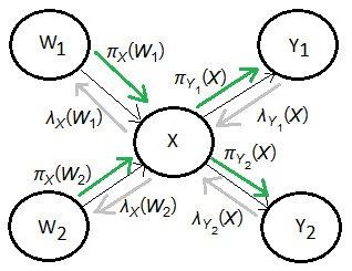
Causal polytree is the structure to be used in this section, each node might have multiple parents.
[1] Forward propagation
➀the predictive support at $X$ comes from its 2 parents $W_{1}$, $W_{2}$.
[2] Backward propagation
$\pi(x)$…$x\in X$
=$P(x\vert e_{X}^{+})$
=$P(x\vert e_{W_{1}X}^{+},e_{W_{2}X}^{+})\cdot P(x\vert W_{1},W_{2})$
=$P(x\vert e_{W_{1}X}^{+})\cdot P(x\vert e_{W_{2}X}^{+})\cdot P(x\vert W_{1},W_{2})$
=$\sum_{w_{1}}\sum_{w_{2}}P(x\vert e_{W_{1}X}^{+})\cdot P(x\vert e_{W_{2}X}^{+})\cdot P(x\vert w_{1},w_{2})$
=$\sum_{w_{1}}\sum_{w_{2}}\pi_{W_{1}}(x)\cdot\pi_{W_{2}}(x)\cdot P(x\vert w_{1},w_{2})$
➁the generalization of forward propagation at $X$ for $n$ parents:
$\pi(x)$=$\sum_{w_{1},…,w_{n}}\pi_{W_{1}}(x)\cdots\pi_{W_{n}}(x)\cdot P(x\vert w_{1},…,w_{n})$
➂as the forward propagation from $X$ to one of its child, say $Y_{k}$, it will have to combine the forward propagation thus obtain above with the backward propagated evidence from $\{Y_{1},…,Y_{k-1},Y_{k+1},…,,Y_{m}\}$, suppose $X$ has $m$ multiple child nodes.➀the diagnostic support at $X$ comes from its 2 children $Y_{1}$, $Y_{2}$, where $\lambda(x)$=$\lambda_{Y_{1}}(x)\cdot\lambda_{Y_{2}}(x)$, must be splitted into 2 parts to be transfered to $W_{1}$, $W_{2}$, which are $\lambda_{X}(w_{1})$,$\lambda_{X}(w_{2})$.
[Cautions]
➁to diagnose in $W_{1}$ the symptom/evidence backward propagated from $X$:
$\lambda_{X}(w_{1})$
=$P(e_{W_{1}X}^{-}\vert W_{1})$
=$P(e_{X}^{-},e_{W_{2}X}^{+}\vert W_{1})$
=$P(e_{X}^{-}\vert W_{1})\cdot P(e_{W_{2}X}^{+}\vert W_{1})$
=$P(e_{X}^{-}\vert x)\cdot P(x\vert W_{1})\cdot P(e_{W_{2}X}^{+})$
=$P(e_{X}^{-}\vert x)\cdot P(x\vert W_{1},W_{2})\cdot S_{1}\cdot P(e_{W_{2}X}^{+})$
=$P(e_{X}^{-}\vert x)\cdot P(x\vert W_{1},W_{2})\cdot S_{2}\cdot P(W_{2}\vert e_{W_{2}X}^{+})$
=$P(e_{X}^{-}\vert x)\cdot P(x\vert W_{1},W_{2})\cdot\beta\cdot P(e_{W_{2}X}^{+}\vert W_{2})$
=$\beta\sum_{x}\lambda(x)\cdot\sum_{w_{2}}P(x\vert w_{1},w_{2})\cdot\pi_{W_{2}}(x)$
, where the $S_{1}$,$S_{2}$,$\beta$ are arbitrary constants to hold the equality. We turn from $P(W_{2}\vert e_{W_{2}X}^{+})$ to $P(e_{W_{2}X}^{+}\vert W_{2})$ to express the deduction in terms of $\pi_{W_{2}}(x)$ for its simplicity.
➂the generalization of $n$ multiple parents:
$\lambda_{X}(w_{i})$
=$\beta\sum_{x}\lambda(x)$
$\;\;\cdot\sum_{w_{k}:k\neq i}P(x\vert w_{1},…,w_{n})$
$\;\;\cdot\prod_{k=1:k\neq i}^{n}\pi_{W_{k}}(x)$The belief updated by propagation would result in expensive computation consumption when there exists multiple parents. The introduction of propagation aims to eliminate the potential expensive computation of NP-hard order in variable elimination, now it seems that it is struggling over. Next to see the clique tree series, to be believed workable in a lot references.
Addendum
➀A T utorial on Bayesian Belief Networks, Mark L Krieg, Surveillance Systems Division Electronics and Surveillance Research Laboratory, DSTO-TN-0403
➁Lecture 4: Probability Propagation in Singly Connected Bayesian Networks, Duncan Fyfe Gillies, Department of Computing Imperial College London


