The Bayesian Network Propagation And Clique Tree
25 Sep 2018Prologue To The Bayesian Network Propagation And Clique Tree
The Clique Tree
A clique tree is an undirected tree, where:
➀each node in the tree is a set of variables, called a clique.
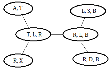
➁if one variable appears in 2 cliques, it must exist in all the cliques in the path between the 2 cliques. It is variable-connected.
This is an invalid clique tree, variable B should exist in all the cliques in the path in between cliques of $(B,S)$ and $(R,D,B)$.
This is a valid clique tree, since it meets the criteria that a variable could be found on all cliques in the path between 2 cliques containing it.
A clique tree covers a Bayesian network if below conditions are meet:
➀the union of the cliques is the set of the variables in the Bayesian network.
➁for any variable $X$, the clique tree has one clique containing this variable with all its parent variables, such clique is called the family cover clique of $X$.
Suppose we are given above Bayesian network, below clique tree is just one such example.
The Clique Tree For Variable Elimination
Supposed we are given this Bayesian network and would like to make the posterior belief update of all variables based on the observed evidence. This paragraph will guide you through the whole process by using the clique tree.
[1] Initialize the cliques with independence probability distribution of BN variablesFor each variable $X$ in Bayesian network:
[2] Instantiate the variable with the observed evidence
➀find the probability of $P(X\vert Pa(X))$ and attach it onto the clique containing $X$.
➁if the clique has no probability of independence attached, set it to the identity function.
Trivially, the multiplication of all functions on the clique tree is equivalent to the full joint probability distribution in the Bayesian network.
Using the same Bayesian network, we denote the observed evidence as $E$, in the real world, we can have observation of multiple variables at the same time.
Suppose we have observed $A=y$ and $X=y$, to instantiate the clique tree, we associate the independence probability function containing $A$ and $X$ with the observed value $y$.
[3] Choose pivot for reference
If we take $\chi$ to be all unobserved variables, $P(\chi,E)$ is just the multiplication of all functions on the clique tess, which will laterly be proved.
➀for one query variable case, choose the clique containing that variable in it to be the pivot.
[4] Pass the messages from the leafs to the pivot
Suppose we’d like to query for $P(L\vert A=y,X=y)$, based on the observation of $A=y,X=y$, in the same example, take the clique $(R,L,B)$ to be the pivot, the $(T,L,R)$ could also be the candidate.
➁for case of two query variables, then combine the cliques of the queried variable together as the pivot, or just choose the clique containing these 2 queried variables, if any exists.
Suppose we’d like to query for $P(T,L\vert A=y,X=y)$, we can directly take the clique $(T,L,R)$ as to pivot. If we’d like to query for $P(T,B\vert A=y,X=y)$, then combine the cliques $(T,L,R)$,$(R,L,B)$ just holds.
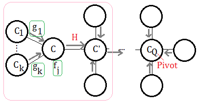
➂for multiple query variables case, follow ➁’s fashion, could we reach the goal.When we have a clique tree constructed, the messages(evidence) are passed from the leafs to the pivot node. Supposed we have such example of undirected graph, the clique is expressed by uppercase C for better understanding.
[5] Posterior belief update
This exhibition reveals the portion mostly closed to the target pivot $C_{Q}$, the messages are coming from $C_{i}$, where $i$=$1$ to $k$, such message passing are triggered by the observed evidence on leaf nodes, maybe far away from these $C_{i}$s.
➀$g_{i}$ is the message from $C_{i}$ to $C$.
➁$f_{j}$ is the function attached to $C$.
➂the messages passed to $C$, are trsnafered to $C’$, we denote it $H$.
$H((C\cap C’)-E)$=$\sum_{C\backslash C’\cup E}\prod_{i}g_{i}\prod_{j}f_{j}$
The summation over elements purely from $C$, not belonging to $C’$ and $E$(evidence).
The term $(C\cap C’)-E$ is better understood by this illustration. Since $C$ and $C'$ are independent, the intersection of the 2 nodes is null. It’s the evidence existing in the space in between $C$ and $C'$, after we minus $E$, what we want is the pure message from $C$ to $C'$.
Supposed we’d like to query for $P(Q|E=e)$ in above given graph of clique tree, and we take $H(Q,\chi)$ to be the function attached or send to $C_{Q}$, where $\chi$ stands for all unobserved variables other than $Q$ in $C_{Q}$:
$P(Q|E=e)$=$\frac {\sum_{\chi}H(Q,\chi)}{\sum_{Q,\chi}H(Q,\chi)}$
Posterior Belief Update Illustration In Clique Tree
[Question][Answer]Using the same clique tree, suppose we are given the observed evidence on $A=y$ and $X=y$, we’d like to make inference on $P(L\vert A=y,X=y)$.
Let’s illustrate by this graph, similar to variable elimination process.
➀do the join over $A=y$ in clique $(A,T)$:
$f_{1}(T)$=$P(A=y)\cdot P(T\vert A=y)$
➁directly take the only attached function in clique $(R,X)$:
$f_{2}(R)$=$P(X=y\vert R)$
➂do the join over $S$ in clique $(L,S,B)$, we’d like to move toward the pivot:
$f_{3}(L,B)$=$\sum_{S}P(S)\cdot P(L\vert S)\cdot P(B\vert S)$
➃do the join over $D$ in clique $(R,D,B)$, we’d like to move toward the pivot:
$f_{4}(R,B)$=$\sum_{D}P(D\vert R,B)$
➄in clique $(T,L,R)$, collect the message from clique $(A,T)$ and $(R,X)$, pass it to the pivot:
$f_{5}(L,R)$=$\sum_{T}f_{1}(T)\cdot f_{2}(R)\cdot P(R\vert T,L)$
This time, join over $T$.
➅thus we have $f_{3}(L,B)$,$f_{4}(R,B)$ and $f_{5}(L,R)$, the joint probability is thus distributed and expressed as:
$H(R,L,B)$=$f_{3}(L,B)\cdot f_{4}(R,B)\cdot f_{5}(L,R)\cdot 1$Finally, $P(L\vert A=y,X=y)$=$\frac {\sum_{R,B}H(R,L,B)}{\sum_{R,L,B}H(R,L,B)}$, since $H(R,L,B)$ already encompass $A=y$ and $X=y$ in it.
The Clique Tree Propagation Algorithm: Computation Sharing In All Queries
[1] The algorithm of two sweep message passing➀the first sweep is collection, from the leafs to the pivot, above posterior belief update illustration is the example.
[2] Propagation from the pivot to the leafs
➁the second sweep is distribution, from the pivot to the leafs. Next to illustrate it.Just like your eyes see somthing, stimulation from certain observation of evidence to the brain, next would be the inspiration from the brain central point back to each distinct parts that had joined in this message frowarding process, finally back to your eyes. This explains why human sometimes tracks object movement, maybe.
Using the same example of clique tree, the message is distributed from the pivot $(R,L,B)$ to all other cliques in reversed direction.
➀$f_{6}(R,L)$=$\sum_{B}f_{3}(L,B)\cdot f_{4}(R,B)\cdot 1$
Combine the $f_{3}(L,B)$,$f_{4}(R,B)$ by joining over $B$, could we have the function of message passing to clique $(T,L,R)$.
➁$f_{7}(R,B)$=$\sum_{L}f_{3}(L,B)\cdot f_{5}(R,L)\cdot 1$
➂$f_{8}(L,B)$=$\sum_{R}f_{4}(R,B)\cdot f_{5}(R,L)\cdot 1$
➃$f_{9}(R)$=$\sum_{T,L}f_{1}(T)\cdot f_{6}(R,L)\cdot P(R\vert T,L)$
Combine $P(R\vert T,L)$ with $f_{1}(T)$ and $f_{6}(R,L)$, join over $T,L$, could we have such expression of the message passing to clique $(R,X)$ from the pivot.
➃$f_{10}(T)$=$\sum_{R}f_{2}(R)\cdot f_{6}(R,L)$Have you found that the function of the message from the pivot to the leafs are all expressed in terms of the variables the same as it is in the clique from which passes message to the pivot.
[3] Posterior belief update after distribution::mjtsai1974Suppose you’d like to infer $P(L\vert A=y,X=y)$ in $(T,L,R)$, since we have $f_{1}(T)$,$f_{2}(R)$,$f_{6}(R,L)$ send to $(T,L,R)$ and $P(R\vert T,L)$ attached to it:
➀$I(T,L,R)$
=$\sum_{B}f_{1}(T)\cdot f_{2}(R)\cdot$
$\;\;f_{3}(L,B)\cdot f_{4}(R,B)\cdot P(R\vert T,L)$
=$f_{1}(T)\cdot f_{2}(R)\cdot f_{6}(R,L)\cdot P(R\vert T,L)$
, where $f_{6}(R,L)$ is the join of $f_{3}(L,B)$ and $f_{4}(R,B)$ over $B$.
➁$P(L\vert A=y,X=y)$
=$\frac {\sum_{T,L,R}I(T,R)}{\sum_{T,L,R}I(T,L,R)}$
➂by using $H(R,L,B)$ or $I(T,L,R)$ is to calculate $P(L\vert A=y,X=y)$ on the same sets of functions!This is my explain of computation sharing.
The Clique Tree Properties
[Property 1] The arguemnts of the functions attached or send to a clique are all veriables in the cliqueIn mjtsai’s explain:
proof::mjtsai1974
➀before $C$ sends to $C’$, the arguments of the functions attached to $C$ or send to $C$ would be passed to a clique $C’$ are all variables in the clique $C$.
➁after $C$ sends to $C’$, the arguments of the functions attached to $C$ or send to $C$ has been passed to a clique $C’$ are all variables in the clique $C$.
Using the same clique tree in above paragraph, focus on the left pink marked part.
[Property 2] Product of functions attached to or send to all un-activated cliques=$P(\chi,E=e)$, where $\chi$ stands for all unobserved variables in these un-activated cliques proof::mjtsai1974
➀by given we have $f_{j}$ attached to $C$ and passing message of $g_{i}$ from $C_{i}$.
➁the function of the messgae from $C$ to $C’$ is thus defined:
$H((C\cap C’)-E)$=$\sum_{C\backslash C’\cup E}\prod_{i}g_{i}\prod_{j}f_{j}$
therefore, the arguments of the functions in the passing messgae from $C$ to $C’$ are all the variables in $C$.We denote a clique is un-activated if it has not send out messages.
Using the same clique tree in below paragraph.
➀take $\chi$ to be the set of unobserved variables in all un-activated cliques, before $C$ send message to $C’$.
➁take $\chi’$ to be the set of unobserved variables in all un-activated cliques, after $C$ send message to $C’$.
➂take $r$ to be the product of functions attached to or send to all un-activated cliques, after $C$ send message to $C’$, then $r$ is a function of $\chi’$, that is $r(\chi’)$, where $H$ is not included, since $H$ is just the function of message passing in between!!
➃consider the message passing from $C$ to $C’$, take $C\backslash C’\cup E$ into account, for simplicity, treat $Z$=$C\backslash C’\cup E$, where $Z\in C$ and $Z\not\in C’$ is of no doubt.
➄under ➃, we have $\chi$=$Z\cup\chi'$, the full illustration is exhibited below:
➅suppose property 2 is true that
$r(\chi’)\cdot\prod_{i}g_{i}\prod_{j}f_{j}$=$P(\chi,E=e)$, next, consider the time point of "before being after"(by $H$) and "being after"(by $r(\chi’)$) $C$ send messages to $C’$, the combinatory of these two distributions provides a full image of distribution in this cliquer tree for the whole "after" $C$ send messages to $C'$:
$r(\chi’)\cdot H((C\cap C’)-E)$
=$r(\chi’)\cdot\sum_{C\backslash C’\cup E}\prod_{i}g_{i}\prod_{j}f_{j}$
=$\sum_{Z}r(\chi’)\cdot\prod_{i}g_{i}\prod_{j}f_{j}$
=$\sum_{Z}P(\chi,E=e)$
=$\sum_{Z}P(Z,\chi’,E=e)$
=$P(\chi’,E=e)$
➆$r(\chi’)\cdot\prod_{i}g_{i}\prod_{j}f_{j}$=$P(\chi,E=e)$
$\Leftrightarrow$
$r(\chi’)\cdot H((C\cap C’)-E)$=$P(\chi’,E=e)$That is to say before $C$ send messages to $C'$, the product of all functions attached to or send to all un-activated cliques(at this moment, $C$, $C'$ and others are all un-activated) and after $C$ send messages to $C'$, the the product of all functions attached to or send to all un-activated cliques(at this moment, $C'$ and others are all un-activated) are all equivalent to: $P(Unobserved\;vars,E=e)$…by mjtsai1974.

