Partial Observable Markov Decision Process - Part 3
10 Oct 2020Prologue To Partial Observable Markov Decision Process - Part 3
POMDP Value Function
[1] Bellman equation for POMDP➀$V^{\ast}(b)$=$max_{a}\{\rho(b,a)$+$\gamma\cdot\int_{b^{'}}P(b^{'}\vert a,b)\cdot V^{\ast}(b^{'})db^{'}\}$
, this expression is in rather intuition, where $\rho(b,a)$=$\sum_{s}R(s,a)\cdot b(s)$, and why integrate over $b^{'}$?
Because the continuous belief update in POMDP.➁$V^{\ast}(b)$=$max_{a}\{\rho(b,a)$+$\gamma\cdot\sum_{b^{'}}P(b^{'}\vert a,b)\cdot V^{\ast}(b^{'})\}$
, this is a more realistic format, where $P(b^{'}\vert a,b)$=$\sum_{o}\sum_{s^{'}}P(o\vert s^{'},a)\cdot\sum_{s}P(s^{'}|a,b)\cdot b(s)$
, which is the belief transition probability derived from POMDP transition/observation models.Notes must be made that in my article, the uppercase letter stands for the variable, whereas the littlecase letter represents the value in it.
[2] Solving POMDP by value iterationWe take the value iteration in POMDP as:
➀$V_{0}(b)$=$0$ to be initial value of belief $b$
➁$V_{t}(b)$=$max_{a}\{R(b,a)$+$\gamma\cdot\sum_{o}P(o\vert a,b)\cdot V_{t-1}(b^{'})\}$
, where $b^{'}$=state estimated from $(a,b,o)$ at timestamp $t-1$.It is the immediate reward plus the expected discounted value of where we end up, say $b^{'}$ and make observation $o$.
$V_{t}(b)$ means that we have $t$ steps to go from $b$, and $V_{t-1}(b^{'})$ indicates we have $t-1$ steps to go from $b^{'}$, where $b$ has been belief updated to $b^{'}$ by action $a$ and observation $o$.
The scary thing is the value function $V$, defined over an infinite set of belief states, $b$, if we make a loop for all belief states to do this update, ➁, it is just an infinite number of belief states, $b^{'}s$, that would not terminated!!!
Difficulties In Solving POMDP
[Notes] Findings in the belief update of tiger exampleA POMDP is a generalization of MDPs to situations that world states are not fully observable.
Recall in my last article POMDP - Part 2, the tiger example, the full illustration of belief updating by listening, before the agent opens the correct door, it continues to listen until the resulting belief of probability distribution over world states is to be believed converged in each path of sequence of observations.
We have 2 findings:
[Difficulty 1] Memory(POMDP) v.s. memoryless(DMP)
➀the agent has to keep track the history of belief update with respect to observation and action taken in each unique path, we need memory in POMDP.
➁after each action, there is a new belief from prior belief. The belief update process is continuous.POMDP lacks important state information and must be compensated by memory.
The agent needs to learn extraneous information in observation to avoid/try, where such information should be maintained by a memory-based model of the world in order to predict what will happen accurately!!
If the agent has the complete full states, then it can choose optimal actions without memory.
Take two hallways for example, optimal policy might take right for the first, might take left for the first, a memoryless policy could not distinguish between them.
You might ponder why not just use the optimal policy in each state to decide the action that leads to the maximum reward!! Because in POMDP, to make observation after taking an action, we need further to know what state we are ranging from, to estimate such probabilistic observation, we need memory for these belief state information.
If we’d like to get reward $R_{1}$, we might take left given that we are in $S_{1}$, then we need to remember that we are in $S_{1}$ already.
[Difficulty 2] Infinite belief statesIn the belief update illustration of tiger example in POMDP - Part 2, you can realize that new belief is generated from prior belief upon action taken, observation made, such process is in a continuous manner.
If we continue to listen in this simple tiger example, over and over, the set of belief states would definitely grow up in its size. To be believe in other application with high complexity, it will be infinite, uncountable.
Then, we should jump from infinity to finite. Value iteration updates couldn't be carried out, because uncountable number of belief state.
Policy Tree
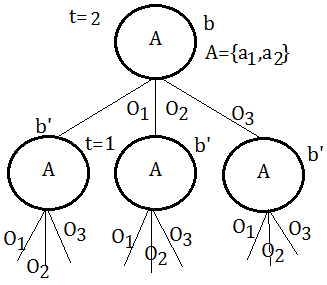
[1] Brief descriptionIn general, an agent-step policy can be represented as a policy tree:
➀search over sequences of actions with limited look-ahead
➁branching over actions and observations
Suppose we begin from root node of certain action $A$, with probabilitistic distribution over observations $\{O_{1},O_{2},…,O_{K}\}$, and totally $H$ steps to go.
With 2 steps to go, it takes an action, make an observation, and make the final action.
With 1 step remaining, the agent must then just take an action and get the immediate reward.
In above tree, there are totally $\vert A\vert^{\frac {\vert O\vert^{H} - 1}{\vert O\vert - 1}}$ nodes.
[2] Relate value function with policy tree[3] Optimal $t$-steps policy
Value function of a policy tree
➀if $P_{t}$ is 1-step policy tree, the value of executing that action in state $s$:
$V_{P_{t}}(s)$=$R(s,a(P_{t}))$, $t=1$
➁if $P_{t}$ is t-steps policy tree, then
$V_{P_{t}}(s)$
=$R(s,A(P_{t}))$+$\gamma\cdot\{Expected\;future\;value\}$
=$R(s,A(P_{t}))$+$\gamma\cdot(\sum_{s^{'}}P(s^{'}\vert b,a)\cdot b(s)$
$\;\;\cdot(\sum_{o}P(o\vert s^{'},a)\cdot V_{O(A(P_{t-1}))}(s^{'})))$
, where we have next $b^{'}$ probabilistically distributed over $s^{'}$
, and $A(P_{t})$=$a$, the action taken in the root node
, with $\sum_{o}P(o\vert b,a)\cdot V(b^{'})$=$\sum_{s^{'}}P(s^{'}\vert b,a)\cdot b(s)$
$\;\;\;\;\cdot(\sum_{o}P(o\vert s^{'},a)\cdot V_{O(A(P_{t-1}))}(s^{'}))$
, and $V_{O(A(P_{t-1}))}(s^{'})$ stands for the value function of $s^{'}$ due to observation as a result of action taken in root node of next $t-1$ steps policy tree.Value function over belief state
➀we could think $V_{P_{t}}(b)$ as a vector associated with the policy tree of $t$-steps, where $dim(V_{P_{t}}(b))$=$n$, for $b$=$\{s_{1},s_{2},…,s_{n}\}$
➁use the notation $\alpha_{P_{t}}$=$\left\langle V_{P_{t}}(s_{1}),V_{P_{t}}(s_{2}),…,V_{P_{t}}(s_{n})\right\rangle$
➂treat value function of belief state $b$ with regard to the $t$-steps policy tree as $V_{P_{t}}(b)$=$\sum_{s}V_{P_{t}}(s)\cdot b(s)$
➃we have $V_{P_{t}}(b)$=$b\cdot\alpha_{P_{t}}$…dot productTo construct an optimal $t$-steps policy, we must maximize over all $t$-steps policy tree $P_{t}$:
$V_{t}^{\ast}(b)$=$max_{\alpha_{p}\in\alpha_{\tau}}\alpha_{p}\cdot b$, where $\alpha_{\tau}$ is a collection of $\alpha_{P_{t}}$As $V_{P_{t}}(b)$ is linear in $b$ for each vector in $\alpha_{\tau}$, then $V_{t}^{\ast}(b)$ would be the upper surface of these functions.
That is to say $V_{t}^{\ast}(b)$ is piecewise linear and convex.
Illustration Of PWLC(Piecewise Linear Convex)
[1] The preliminary[2] $1$-step POMDP value function
The given scenario
Suppose we are given the world of 2 states, 2 actions and each action taken might lead to 3 possible observations in this environment of uncertainty.$V_{P_{t}(a_{i})}$
Let $V_{P_{t}(a_{i})}$ to be the value function induced by policy tree $P_{t}$, with $a_{i}$ the $i$-th action in the root node, and this value function is of the form:
$\;\;V_{P_{t}(a_{i})}(b)$=$b\cdot\alpha_{P_{t}}(a_{i})$It is a multi-linear function of $b$, for each value function could be shown as a line, plan, or hyperplan, depends on the number of states.
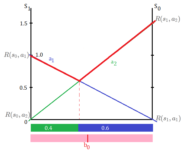
For $1$-step policy tree, we just take one single action and get the immediate reward to be the value function, such immediate reward due to action execution is over $s_{0}$ and $s_{1}$, weighted by the initial belief distribution, with respect to $a_{1}$ and $a_{2}$ each:
➀$R(a_{1},b)$=$\{R(s_{0},a_{1}),R(s_{1},a_{1})\}$
➁$R(a_{2},b)$=$\{R(s_{0},a_{2}),R(s_{1},a_{2})\}$[3] $2$-steps POMDP value function
The induction of $1$-step POMDP value function
$V_{P_{t}(a_{i})}(b)$=$\sum_{s}R(s,a_{i})\cdot b(s)$, for $s\in\{s_{0},s_{1}\}$, given that $b_{0}\lbrack 0.5\;0.5\rbrack$, and immediate rewards are initialized as shown, then
➀$V_{P_{1}(a_{1})}(b)$
=$R(s_{0},a_{1})\cdot b(s_{0})$+$R(s_{1},a_{1})\cdot b(s_{1})$
=$1\cdot 0.5$+$0\cdot 0.5$
=$0.5$
➁$V_{P_{1}(a_{2})}(b)$
=$R(s_{0},a_{2})\cdot b(s_{0})$+$R(s_{1},a_{2})\cdot b(s_{1})$
=$0\cdot 0.5$+$1.5\cdot 0.5$
=$0.75$The linearity
Since $V_{P_{t}(a_{i})}(b)$ is linear in $b$, therefore we have
$\begin{bmatrix}R(s_{0},a_{1})&R(s_{1},a_{1})\\R(s_{0},a_{2})&R(s_{1},a_{2})\end{bmatrix}\begin{bmatrix}b(s_{0})\\b(s_{1})\end{bmatrix}=\begin{bmatrix}V_{P_1(a_1)}(b)\\V_{P_1(a_2)}(b)\end{bmatrix}$
$\Rightarrow\begin{bmatrix}1&0\\0&1.5\end{bmatrix}\begin{bmatrix}b(s_{0})\\b(s_{1})\end{bmatrix}=\begin{bmatrix}0.5\\0.75\end{bmatrix}$, just holds
The additive of $2$ linear lines leads to PWLC at $t$=1.Find out the intersection point
This turns to solve $V_{P_{1}(a_{1})}(b)$=$V_{P_{1}(a_{2})}(b)$,
$\Rightarrow R(s_{0},a_{1})\cdot b(s_{0})$+$R(s_{1},a_{1})\cdot b(s_{1})$
=$R(s_{0},a_{2})\cdot b(s_{0})$+$R(s_{1},a_{2})\cdot b(s_{1})$
$\Rightarrow 1\cdot b(s_{0})$+$0\cdot b(s_{1})$=$0\cdot b(s_{0})$+$1.5\cdot b(s_{1})$
After the deductio by $b(s_{0})$=$1-b(s_{1})$, we have $b(s_{0})$=0.6 and $b(s_{1})$=$0.4$Find out the optimal action
➀by maximizing over $1$-step policy tree $P_{1}$, we have optimal action probabilistically distributed in proportion to the region partitioned at this intersection point.
➁this optimal $1$-step policy is determined by projecting the optimal value function back down to the belief space.
➂such projection yields a partition into regions, within each distinct region, there is a policy tree, say $P_{t}(a_{i})$, $t$=$1$ for horizon $1$, by taking action of $a_{i}$ leads us to the maximum of value function in this region.
➃in this $1$-step policy tree, we have $a_{1}$ to be the optimal action in $\lbrack 0\;0.4\rbrack$ interval of belief space, and within $\lbrack 0.4\;1\rbrack$ interval, we have $a_{2}$ the optimal action in above exhibition.
- Why do we have $s_{0}$ axis consisting of $R(s_{1},a_{i})$?
$\because b(s_{1})$=$1-b(s_{0})$
$\therefore R(s_{1},a_{i})$ for $i=\{1,2\}$ in this example whould we have $s_{0}$ as the departuring point, extend the width with the portion to $1-b(s_{0})$, where the $s_{0}$ ranging in the opposite direction, heading toward $s_{1}$ axis. Similarity could be found in axis of $s_{1}$.[4] $3$-steps POMDP value function
The general format
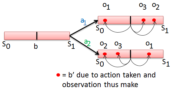
➀with 2 steps to go, we can take an action, make observation, then take next one left action base on the observation.
➁the $2$-steps POMDP value function is obtained by adding the immediate reward of 1-st action taken, plus the value of taking next one left action, such expression is of the form:
$V_{P_{2}(a_{i})}(b)$
=$V_{2}(b)$…for simplicity
=$R(a_{i},b)$+$\gamma\cdot\{expected\;future\;value\}$
=$R(a_{i},b)$+$\gamma\cdot\sum_{o_{j}}P(o_{j}\vert b,a_{i})\cdot V_{1}(b^{'})$
, where we have belief update from $b$ to $b^{'}$ due to action $a_{i}$, observation $o_{j}$, and we write $V_{P_{2}(a_{i})}(b)$ as $V_{2}(a_{i},b)$ or $V_{2}(b)$.
- Value function transformation
➀the horizon $2$ value function is a function of next belief $b^{'}$, since by taking action $a$, with certain observation, would this initial/prior belief $b$ be updated to $b^{'}$. As a result, that we have the horizon $2$ value function:
$V_{2}(b)$
=$max_{a}\{R(a,b)$+$\gamma\cdot\sum_{o_{j}}P(o_{j}\vert b,a)\cdot V_{1}(b^{'})\}$
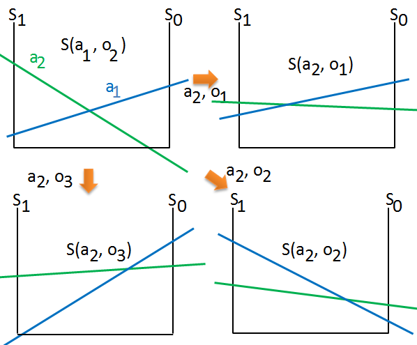
, where $P(o_{j}\vert b,a)\cdot V_{1}(b^{'})$ is the horizon $1$ value function transformation denoted as $S(a,o_{j})$, each $o_{j}$ has its own transformed alpha vectors.
➁the transformed/next belief $b^{'}$ is a function of the initial/prior belief $b$:
$b^{'}(S^{'})$
=$P(S^{'}|A,O,b)$, we believe we are in state $S^{'}$, given observation $O$
=$\frac {P(O|S^{'},A,b)\cdot P(S^{'}|A,b)}{P(O|A,b)}$- The induction of $2$-steps POMDP value function
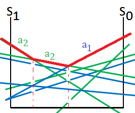
➀there are 2 actions in this example, we begin by extending from $a_{1}$ at $t$=$2$:
➁combine these linear lines together we get:
➂by pruning and partioning we can get the optimal actions in each region:
➃we next extend from $a_{2}$ at $t$=$2$, suppose we get optimal action of region partitioned in below:
➄put it all together, we could get the optimal actions as a whole image:
Suppose we are inheriting from above optimal actions in PWLC format of horizon $2$, such paths are listed below:
➀take action $a_{1}$, make observation $o_{2}$, then make action $a_{2}$(could be mapped from above graph)
➁take action $a_{2}$, make observation $o_{1}$, then make action $a_{2}$
➂take action $a_{2}$, make observation $o_{3}$, then make action $a_{1}$
, where ➁ and ➂ are not exhibitted, for I directly make assumption of start from $a_{1}$ for simplicity.It would be a little complicated to ask for the value function of $3$-steps POMDP, we should just follow the path leading to the optimal action in prior $2$-steps policy tree.
The general format recap
The general format of value function in POMDP is
$V_{t}(b)$
=$max_{a}\{ R(a,b)+\gamma\cdot\sum_{o_{j}}P(o_{j}\vert a,b)\cdot V_{t-1}(b^{'})\}$
, where we make belief update from $b$ to $b^{'}$, due to action $a$, with observation $o_{j}$, and we get the resulting $V_{t-1}(b^{'})$ with regard to each of this path, and $t=3$ in this section now.The value function persists in transformation
The value function transformation continues to apply on the last end node in above $2$-steps policy tree, for each distinct path, say from the very last $S(a_{1},o_{2})$, to turn into $S(a_{2},o_{1})$,$S(a_{2},o_{2})$,$S(a_{2},o_{3})$. We are following the path $1$-st action $a_{1}$, make observation $o_{2}$, then $2$-nd action $a_{2}$:
The induction of $3$-steps POMDP value function
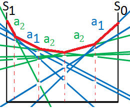
➀combine these linear lines together, by pruning and partioning we can get the optimal actions in each region:
➁we then start from the path of $1$-st action $a_{2}$, make observation $o_{1}$, then $2$-nd action $a_{2}$, for simplicity, we get below optimal actions in each region:
➂we next start from the path of $1$-st action $a_{2}$, make observation $o_{3}$, then $2$-nd action $a_{1}$, for simplicity, we get below optimal actions in each region:
➃put it together, we could get the optimal action partitions in below:
Addendum
➀Partial Observable Markov Decision Process, Charles IsBell, Michael Littman, Reinforcement Learning By Georgia Tech(CS8803)
➁POMDP Value Iteration Example, Tony, Brown University’s Computer Science Department
➂POMDP Tutorial, Stefan Kopp, Bielefeld University
➃POMDPOs, Rowan McAllister and Alexandre Navarro, MLG Reading Group, 02 June 2016, Cambridge University

