04 Dec 2020
Prologue To Partial Observable Markov Decision Process - Part 4
This post will explain why PWLC works and how it is aggregated in value iteration of POMDP(Partial Observable Markov Decision Process).
Recap POMDP Value Iteration
-
Basic idea in POMDP value iteration
➀calculate value function vectors for each action with regard to observation thus made in horizon $1$.
➁continue looking forward horizon $2$,$3$,…
➂make such value iteration until convergence
-
The PWLC(piecewise linear convex)
The value function of POMDP can be represented as max of linear segments - PWLC.
$\left(1\right)$convexity:
state is known at the edges of belief space
$\left(2\right)$linear segments:
➀linear function in the format of belief $\times$ reward
➁segments in horizon 1 are linear
➂segments in horizon $n$ are linear combination of horizon $n-1$'s segments
Illustration: Why And How PWLC Works?
In this section, I am going to lead you to the reason to why PWLC takes effect, and guide you through the way it is aggregated to a convergence.
The value function of POMDP can be represented as max of linear segments - PWLC could be expressed:
$V_{t}(b)$
=$max_{\alpha\in\tau_{t}}\alpha\cdot b$
=$max_{\alpha\in\tau_{t}}\sum_{s}\alpha(s)\cdot b(s)$
[Question]
Assume we have $\tau_{t-1}$ such that $V_{t-1}(b)$=$max_{\alpha\in\tau_{t-1}}\alpha\cdot b$, you are ask to build $\tau_{t}$ such that $V_{t}(b)$=$max_{\alpha\in\tau_{t}}\alpha\cdot b$
[Answer]
-
proof::part-1
➀$V_{t}(b)$=$max_{a\in A}V_{t}^{a}(b)$
$\Rightarrow V_{t}^{a}(b)$=$\sum_{o}V_{t}^{a,o}(b)$
$\Rightarrow V_{t}^{a,o}(b)$=$\sum_{s}R(s,a)\cdot\frac {b(s)}{\left|o\right|}$+$\gamma\cdot P(o\vert b,a)\cdot V_{t-1}(S.E(b,a,o))$
, where we have
$V_{t-1}(S.E(b,a,o))$
=$max_{\alpha\in\tau_{t-1}}\sum_{s^{'}}\alpha(s^{'})\cdot\frac {P(o\vert s^{'},a)\cdot\sum_{s}P(s^{'}\vert s,a)\cdot b(s)}{P(o\vert b,a)}$
➁although $V_{t-1}(S.E(b,a,o))$ is highly non-linear, its awasome denominator part of $P(o\vert b,a)$ could be safely eliminated and tossed out, thus we are left with a linear transformation from $V_{t}^{a,o}(b)$ to its next $V_{t-1}(S.E(b,a,o))$, and $S.E(b,a,o)$=$b^{'}$, which strongly supports value function transformation in Illustration Of PWLC(Piecewise Linear Convex) in POMDP - Part 3.
-
proof::part-2
Succeeding to part-1,
$\tau_{t}$=$U_{a}\tau_{t}^{a}$
$\tau_{t}^{a}$=$\oplus\tau_{t}^{a,o}$
$\Leftrightarrow V_{t}^{a}(b)$=$\sum_{o}V_{t}^{a,o}(b)$
, where we have
➀finite state space, action space, observation space
➁$\left|A\right|\times\left|O\right|$ could be quiet big, but, it is finite.
➂$\left|\tau_{t}\right|$ could grow up doubly, exponentially with $t$, but, it is finite.
We have $\left|\tau_{t}\right|$=$\left|\tau_{t-1}\right|^{\left|O\right|}\times\left|A\right|$
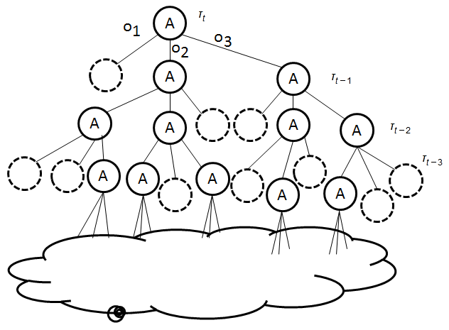
$\tau_{t}$ is derived from the vectors of optimal actions, associated with the dedicated observation in $\tau_{t-1}$.
The POMDP Value Iteration Drawbacks
➀time complexity is exponential in actions and observations.
➁dimensionality of belief space grows with state numbers.
➂exponential growth with number of iterations.
Hugely intractable to solve optimality, value iteration aims for small POMDP problems.
Addendum
➀Partial Observable Markov Decision Process, Charles IsBell, Michael Littman, Reinforcement Learning By Georgia Tech(CS8803)
➁POMDP Value Iteration Example, Tony, Brown University’s Computer Science Department
➂POMDP Tutorial, Stefan Kopp, Bielefeld University
➃Partially Observable Markov Decision Process, Geoff Hollinger, 2007 fall
➄POMDPOs, Rowan McAllister and Alexandre Navarro, MLG Reading Group, 02 June 2016, Cambridge University
10 Oct 2020
Prologue To Partial Observable Markov Decision Process - Part 3
This post will begin with the difficulties in solving POMDP(Partial Observable Markov Decision Process), guide you througth the illustration of value iteration, and lead you to one of the canonical approach of the PWLC(piecewise linear convex).
POMDP Value Function
[1]
Bellman equation for POMDP
➀$V^{\ast}(b)$=$max_{a}\{\rho(b,a)$+$\gamma\cdot\int_{b^{'}}P(b^{'}\vert a,b)\cdot V^{\ast}(b^{'})db^{'}\}$
, this expression is in rather intuition, where $\rho(b,a)$=$\sum_{s}R(s,a)\cdot b(s)$, and why integrate over $b^{'}$?
Because the continuous belief update in POMDP.
➁$V^{\ast}(b)$=$max_{a}\{\rho(b,a)$+$\gamma\cdot\sum_{b^{'}}P(b^{'}\vert a,b)\cdot V^{\ast}(b^{'})\}$
, this is a more realistic format, where $P(b^{'}\vert a,b)$=$\sum_{o}\sum_{s^{'}}P(o\vert s^{'},a)\cdot\sum_{s}P(s^{'}|a,b)\cdot b(s)$
, which is the belief transition probability derived from POMDP transition/observation models.
Notes must be made that in my article, the uppercase letter stands for the variable, whereas the littlecase letter represents the value in it.
[2]
Solving POMDP by value iteration
We take the value iteration in POMDP as:
➀$V_{0}(b)$=$0$ to be initial value of belief $b$
➁$V_{t}(b)$=$max_{a}\{R(b,a)$+$\gamma\cdot\sum_{o}P(o\vert a,b)\cdot V_{t-1}(b^{'})\}$
, where $b^{'}$=state estimated from $(a,b,o)$ at timestamp $t-1$.
It is the immediate reward plus the expected discounted value of where we end up, say $b^{'}$ and make observation $o$.
$V_{t}(b)$ means that we have $t$ steps to go from $b$, and $V_{t-1}(b^{'})$ indicates we have $t-1$ steps to go from $b^{'}$, where $b$ has been belief updated to $b^{'}$ by action $a$ and observation $o$.
The scary thing is the value function $V$, defined over an infinite set of belief states, $b$, if we make a loop for all belief states to do this update, ➁, it is just an infinite number of belief states, $b^{'}s$, that would not terminated!!!
Difficulties In Solving POMDP
[Notes]
Findings in the belief update of tiger example
A POMDP is a generalization of MDPs to situations that world states are not fully observable.
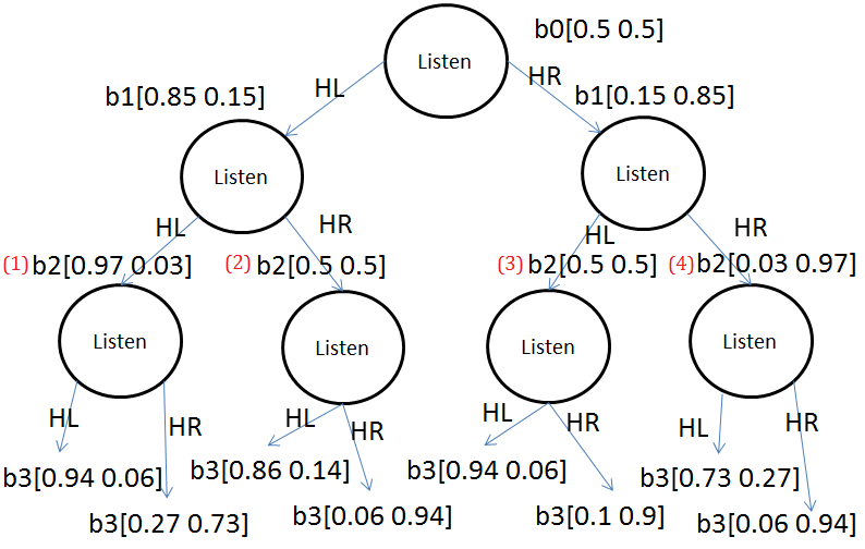
Recall in my last article POMDP - Part 2, the tiger example, the full illustration of belief updating by listening, before the agent opens the correct door, it continues to listen until the resulting belief of probability distribution over world states is to be believed converged in each path of sequence of observations.
We have 2 findings:
➀the agent has to keep track the history of belief update with respect to observation and action taken in each unique path, we need memory in POMDP.
➁after each action, there is a new belief from prior belief. The belief update process is continuous.
[Difficulty 1]
Memory(POMDP) v.s. memoryless(DMP)
POMDP lacks important state information and must be compensated by memory.
The agent needs to learn extraneous information in observation to avoid/try, where such information should be maintained by a memory-based model of the world in order to predict what will happen accurately!!
If the agent has the complete full states, then it can choose optimal actions without memory.
Take two hallways for example, optimal policy might take right for the first, might take left for the first, a memoryless policy could not distinguish between them.

You might ponder why not just use the optimal policy in each state to decide the action that leads to the maximum reward!! Because in POMDP, to make observation after taking an action, we need further to know what state we are ranging from, to estimate such probabilistic observation, we need memory for these belief state information.
If we’d like to get reward $R_{1}$, we might take left given that we are in $S_{1}$, then we need to remember that we are in $S_{1}$ already.
[Difficulty 2]
Infinite belief states
In the belief update illustration of tiger example in POMDP - Part 2, you can realize that new belief is generated from prior belief upon action taken, observation made, such process is in a continuous manner.
If we continue to listen in this simple tiger example, over and over, the set of belief states would definitely grow up in its size. To be believe in other application with high complexity, it will be infinite, uncountable.
Then, we should jump from infinity to finite. Value iteration updates couldn't be carried out, because uncountable number of belief state.
Policy Tree
[1]
Brief description
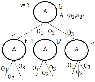
In general, an agent-step policy can be represented as a policy tree:
➀search over sequences of actions with limited look-ahead
➁branching over actions and observations
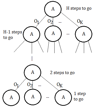 Suppose we begin from root node of certain action $A$, with probabilitistic distribution over observations $\{O_{1},O_{2},…,O_{K}\}$, and totally $H$ steps to go.
With 2 steps to go, it takes an action, make an observation, and make the final action.
With 1 step remaining, the agent must then just take an action and get the immediate reward.
In above tree, there are totally $\vert A\vert^{\frac {\vert O\vert^{H} - 1}{\vert O\vert - 1}}$ nodes.
[2]
Relate value function with policy tree
-
Value function of a policy tree
➀if $P_{t}$ is 1-step policy tree, the value of executing that action in state $s$:
$V_{P_{t}}(s)$=$R(s,a(P_{t}))$, $t=1$
➁if $P_{t}$ is t-steps policy tree, then
$V_{P_{t}}(s)$
=$R(s,A(P_{t}))$+$\gamma\cdot\{Expected\;future\;value\}$
=$R(s,A(P_{t}))$+$\gamma\cdot(\sum_{s^{'}}P(s^{'}\vert b,a)\cdot b(s)$
$\;\;\cdot(\sum_{o}P(o\vert s^{'},a)\cdot V_{O(A(P_{t-1}))}(s^{'})))$
, where we have next $b^{'}$ probabilistically distributed over $s^{'}$
, and $A(P_{t})$=$a$, the action taken in the root node
, with $\sum_{o}P(o\vert b,a)\cdot V(b^{'})$=$\sum_{s^{'}}P(s^{'}\vert b,a)\cdot b(s)$
$\;\;\;\;\cdot(\sum_{o}P(o\vert s^{'},a)\cdot V_{O(A(P_{t-1}))}(s^{'}))$
, and $V_{O(A(P_{t-1}))}(s^{'})$ stands for the value function of $s^{'}$ due to observation as a result of action taken in root node of next $t-1$ steps policy tree.
-
Value function over belief state
➀we could think $V_{P_{t}}(b)$ as a vector associated with the policy tree of $t$-steps, where $dim(V_{P_{t}}(b))$=$n$, for $b$=$\{s_{1},s_{2},…,s_{n}\}$
➁use the notation $\alpha_{P_{t}}$=$\left\langle V_{P_{t}}(s_{1}),V_{P_{t}}(s_{2}),…,V_{P_{t}}(s_{n})\right\rangle$
➂treat value function of belief state $b$ with regard to the $t$-steps policy tree as $V_{P_{t}}(b)$=$\sum_{s}V_{P_{t}}(s)\cdot b(s)$
➃we have $V_{P_{t}}(b)$=$b\cdot\alpha_{P_{t}}$…dot product
[3]
Optimal $t$-steps policy
To construct an optimal $t$-steps policy, we must maximize over all $t$-steps policy tree $P_{t}$:
$V_{t}^{\ast}(b)$=$max_{\alpha_{p}\in\alpha_{\tau}}\alpha_{p}\cdot b$, where $\alpha_{\tau}$ is a collection of $\alpha_{P_{t}}$
As $V_{P_{t}}(b)$ is linear in $b$ for each vector in $\alpha_{\tau}$, then $V_{t}^{\ast}(b)$ would be the upper surface of these functions.
That is to say $V_{t}^{\ast}(b)$ is piecewise linear and convex.
[1]
The preliminary
-
The given scenario
Suppose we are given the world of 2 states, 2 actions and each action taken might lead to 3 possible observations in this environment of uncertainty.
-
$V_{P_{t}(a_{i})}$
Let $V_{P_{t}(a_{i})}$ to be the value function induced by policy tree $P_{t}$, with $a_{i}$ the $i$-th action in the root node, and this value function is of the form:
$\;\;V_{P_{t}(a_{i})}(b)$=$b\cdot\alpha_{P_{t}}(a_{i})$
It is a multi-linear function of $b$, for each value function could be shown as a line, plan, or hyperplan, depends on the number of states.
[2]
$1$-step POMDP value function
For $1$-step policy tree, we just take one single action and get the immediate reward to be the value function, such immediate reward due to action execution is over $s_{0}$ and $s_{1}$, weighted by the initial belief distribution, with respect to $a_{1}$ and $a_{2}$ each:
➀$R(a_{1},b)$=$\{R(s_{0},a_{1}),R(s_{1},a_{1})\}$
➁$R(a_{2},b)$=$\{R(s_{0},a_{2}),R(s_{1},a_{2})\}$
-
The induction of $1$-step POMDP value function
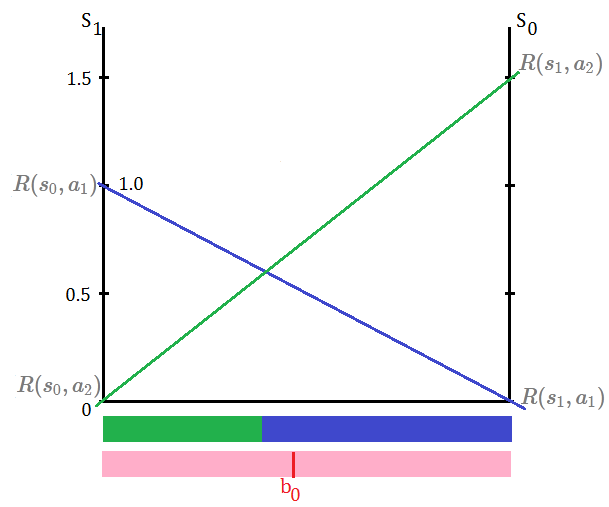 $V_{P_{t}(a_{i})}(b)$=$\sum_{s}R(s,a_{i})\cdot b(s)$, for $s\in\{s_{0},s_{1}\}$, given that $b_{0}\lbrack 0.5\;0.5\rbrack$, and immediate rewards are initialized as shown, then
➀$V_{P_{1}(a_{1})}(b)$
=$R(s_{0},a_{1})\cdot b(s_{0})$+$R(s_{1},a_{1})\cdot b(s_{1})$
=$1\cdot 0.5$+$0\cdot 0.5$
=$0.5$
➁$V_{P_{1}(a_{2})}(b)$
=$R(s_{0},a_{2})\cdot b(s_{0})$+$R(s_{1},a_{2})\cdot b(s_{1})$
=$0\cdot 0.5$+$1.5\cdot 0.5$
=$0.75$
-
The linearity
Since $V_{P_{t}(a_{i})}(b)$ is linear in $b$, therefore we have
$\begin{bmatrix}R(s_{0},a_{1})&R(s_{1},a_{1})\\R(s_{0},a_{2})&R(s_{1},a_{2})\end{bmatrix}\begin{bmatrix}b(s_{0})\\b(s_{1})\end{bmatrix}=\begin{bmatrix}V_{P_1(a_1)}(b)\\V_{P_1(a_2)}(b)\end{bmatrix}$
$\Rightarrow\begin{bmatrix}1&0\\0&1.5\end{bmatrix}\begin{bmatrix}b(s_{0})\\b(s_{1})\end{bmatrix}=\begin{bmatrix}0.5\\0.75\end{bmatrix}$, just holds
The additive of $2$ linear lines leads to PWLC at $t$=1.
-
Find out the intersection point
This turns to solve $V_{P_{1}(a_{1})}(b)$=$V_{P_{1}(a_{2})}(b)$,
$\Rightarrow R(s_{0},a_{1})\cdot b(s_{0})$+$R(s_{1},a_{1})\cdot b(s_{1})$
=$R(s_{0},a_{2})\cdot b(s_{0})$+$R(s_{1},a_{2})\cdot b(s_{1})$
$\Rightarrow 1\cdot b(s_{0})$+$0\cdot b(s_{1})$=$0\cdot b(s_{0})$+$1.5\cdot b(s_{1})$
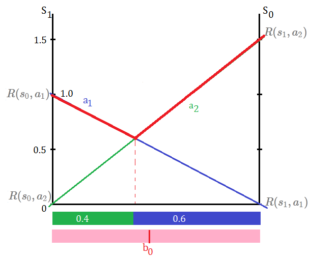
After the deductio by $b(s_{0})$=$1-b(s_{1})$, we have $b(s_{0})$=0.6 and $b(s_{1})$=$0.4$
-
Find out the optimal action
➀by maximizing over $1$-step policy tree $P_{1}$, we have optimal action probabilistically distributed in proportion to the region partitioned at this intersection point.
➁this optimal $1$-step policy is determined by projecting the optimal value function back down to the belief space.
➂such projection yields a partition into regions, within each distinct region, there is a policy tree, say $P_{t}(a_{i})$, $t$=$1$ for horizon $1$, by taking action of $a_{i}$ leads us to the maximum of value function in this region.
➃in this $1$-step policy tree, we have $a_{1}$ to be the optimal action in $\lbrack 0\;0.4\rbrack$ interval of belief space, and within $\lbrack 0.4\;1\rbrack$ interval, we have $a_{2}$ the optimal action in above exhibition.
-
Why do we have $s_{0}$ axis consisting of $R(s_{1},a_{i})$?
$\because b(s_{1})$=$1-b(s_{0})$
$\therefore R(s_{1},a_{i})$ for $i=\{1,2\}$ in this example whould we have $s_{0}$ as the departuring point, extend the width with the portion to $1-b(s_{0})$, where the $s_{0}$ ranging in the opposite direction, heading toward $s_{1}$ axis. Similarity could be found in axis of $s_{1}$.
[3]
$2$-steps POMDP value function
-
The general format
➀with 2 steps to go, we can take an action, make observation, then take next one left action base on the observation.
➁the $2$-steps POMDP value function is obtained by adding the immediate reward of 1-st action taken, plus the value of taking next one left action, such expression is of the form:
$V_{P_{2}(a_{i})}(b)$
=$V_{2}(b)$…for simplicity
=$R(a_{i},b)$+$\gamma\cdot\{expected\;future\;value\}$
=$R(a_{i},b)$+$\gamma\cdot\sum_{o_{j}}P(o_{j}\vert b,a_{i})\cdot V_{1}(b^{'})$
, where we have belief update from $b$ to $b^{'}$ due to action $a_{i}$, observation $o_{j}$, and we write $V_{P_{2}(a_{i})}(b)$ as $V_{2}(a_{i},b)$ or $V_{2}(b)$.
-
Value function transformation
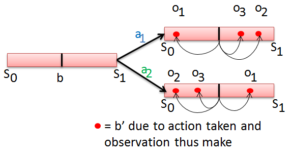
➀the horizon $2$ value function is a function of next belief $b^{'}$, since by taking action $a$, with certain observation, would this initial/prior belief $b$ be updated to $b^{'}$. As a result, that we have the horizon $2$ value function:
$V_{2}(b)$
=$max_{a}\{R(a,b)$+$\gamma\cdot\sum_{o_{j}}P(o_{j}\vert b,a)\cdot V_{1}(b^{'})\}$
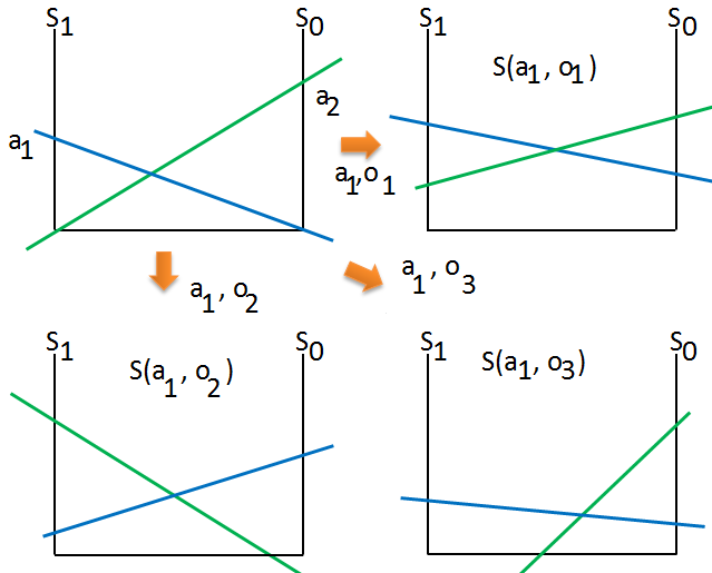
, where $P(o_{j}\vert b,a)\cdot V_{1}(b^{'})$ is the horizon $1$ value function transformation denoted as $S(a,o_{j})$, each $o_{j}$ has its own transformed alpha vectors.
➁the transformed/next belief $b^{'}$ is a function of the initial/prior belief $b$:
$b^{'}(S^{'})$
=$P(S^{'}|A,O,b)$, we believe we are in state $S^{'}$, given observation $O$
=$\frac {P(O|S^{'},A,b)\cdot P(S^{'}|A,b)}{P(O|A,b)}$
- The induction of $2$-steps POMDP value function
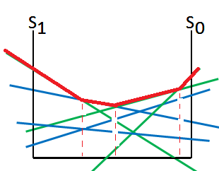
➀there are 2 actions in this example, we begin by extending from $a_{1}$ at $t$=$2$:
 ➁combine these linear lines together we get:
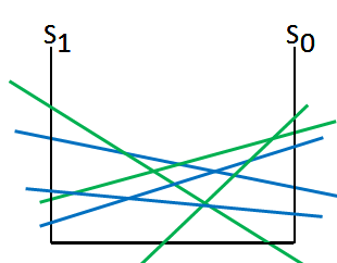 ➂by pruning and partioning we can get the optimal actions in each region:
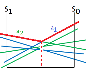
 ➃we next extend from $a_{2}$ at $t$=$2$, suppose we get optimal action of region partitioned in below:
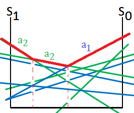
 ➄put it all together, we could get the optimal actions as a whole image:
[4]
$3$-steps POMDP value function
Suppose we are inheriting from above optimal actions in PWLC format of horizon $2$, such paths are listed below:
➀take action $a_{1}$, make observation $o_{2}$, then make action $a_{2}$(could be mapped from above graph)
➁take action $a_{2}$, make observation $o_{1}$, then make action $a_{2}$
➂take action $a_{2}$, make observation $o_{3}$, then make action $a_{1}$
, where ➁ and ➂ are not exhibitted, for I directly make assumption of start from $a_{1}$ for simplicity.
It would be a little complicated to ask for the value function of $3$-steps POMDP, we should just follow the path leading to the optimal action in prior $2$-steps policy tree.
-
The general format recap
The general format of value function in POMDP is
$V_{t}(b)$
=$max_{a}\{ R(a,b)+\gamma\cdot\sum_{o_{j}}P(o_{j}\vert a,b)\cdot V_{t-1}(b^{'})\}$
, where we make belief update from $b$ to $b^{'}$, due to action $a$, with observation $o_{j}$, and we get the resulting $V_{t-1}(b^{'})$ with regard to each of this path, and $t=3$ in this section now.
-
The value function persists in transformation
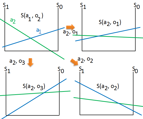
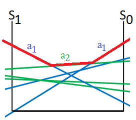
The value function transformation continues to apply on the last end node in above $2$-steps policy tree, for each distinct path, say from the very last $S(a_{1},o_{2})$, to turn into $S(a_{2},o_{1})$,$S(a_{2},o_{2})$,$S(a_{2},o_{3})$. We are following the path $1$-st action $a_{1}$, make observation $o_{2}$, then $2$-nd action $a_{2}$:
-
The induction of $3$-steps POMDP value function
➀combine these linear lines together, by pruning and partioning we can get the optimal actions in each region:
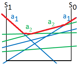
 ➁we then start from the path of $1$-st action $a_{2}$, make observation $o_{1}$, then $2$-nd action $a_{2}$, for simplicity, we get below optimal actions in each region:
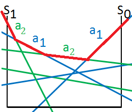
 ➂we next start from the path of $1$-st action $a_{2}$, make observation $o_{3}$, then $2$-nd action $a_{1}$, for simplicity, we get below optimal actions in each region:
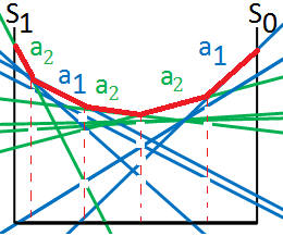
 ➃put it together, we could get the optimal action partitions in below:
Addendum
➀Partial Observable Markov Decision Process, Charles IsBell, Michael Littman, Reinforcement Learning By Georgia Tech(CS8803)
➁POMDP Value Iteration Example, Tony, Brown University’s Computer Science Department
➂POMDP Tutorial, Stefan Kopp, Bielefeld University
➃POMDPOs, Rowan McAllister and Alexandre Navarro, MLG Reading Group, 02 June 2016, Cambridge University
13 Aug 2020
Prologue To Partial Observable Markov Decision Process - Part 2
This post will make a full illustration of belief update in POMDP(Partial Observable Markov Decision Process).
The Real World Is Almost Partially Observable
Policies Under POMDP?
[Question]
Should we use policy mapping state to action in POMDP?
[Answer]
Before we step any further, it strikes on our head that:
➀the agent only gets some(partial) observations
➁no more Markovian signal(the state) directly available to the agent
We should use all information obtained, the full history of observations, by doing the belief update.
Hints On Belief Update
[1]
Calculation
POMDP is often given an initial belief:
➀we are given an initial probability distribution over states in the departure point.
➁we shhould keep track of how this initial probability distribution over states changes from initial point to the next step.
➂by the already known prior belief $b$, the action taken $A$, the observation thus made $O$, to figure out the new next belief $b^{'}$.
This process is called the belief update.
[2]
Apply the Bayer's rule
➀begin from the Bayes Theorem:
$P(B\vert A)$=$\frac {P(A\vert B)\cdot P(B)}{P(A)}$
➁substitute the relevant variables:
$P(S^{'}\vert O)$=$\frac {P(O\vert S^{'})\cdot P(S^{'})}{P(O)}$
➂add the action $A$ and prior belief $b$ in the given:
$P(S^{'}\vert O,A,b)$=$\frac {P(O\vert S^{'},A,b)\cdot P(S^{'}\vert A,b)}{P(O\vert A,b)}$
➃expand $P(S^{'}\vert A,b)$ and $P(O\vert A,b)$
$P(S^{'}\vert O,A,b)$
=$\frac {P(O\vert S^{'},A,b)\cdot P(S^{'}\vert A,b)}{P(O\vert A,b)}$
=$\frac {P(O\vert S^{'},A,b)\cdot \sum_{S}P(S^{'}\vert A,S)\cdot b(S)}{\sum_{S^{''}}P(O|S^{''})\cdot\sum_{S}P(S^{''}|A,S)\cdot b(S)}$
Full Illustration Of Belief Update In Tiger Problem
[1]
The tiger problem
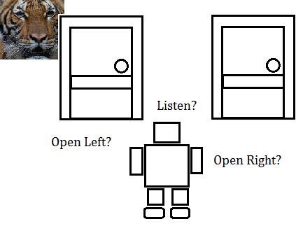
-
The given condition
➀suppose you(the agent) are standing in front of 2 doors, there is a tiger behind one of the 2 doors, that is to say the world states are tiger is behind the left or right door.
➁there are 3 actions, listen, open left door and open right door.
➂listen is not free and might get inaccurate information.
➃when you open the wrong door, you will get eaten by tiger, the reward is $-100$.
➄if you open the right door, you will get $+10$ as the reward.
➅you will get $-1$ after each listen.
-
Transitive probability
➀by listening, the tiger stays where it is.
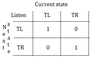 ➁when you open the left door, the tiger has $50%$ to stay behind the left door, or $50%$ to stay behind the right door.
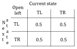
➂when you open the right door, the tiger has $50%$ to stay behind the right door, or $50%$ to stay behind the left door.
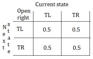
-
Observation and its probability
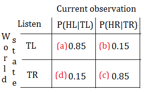
➀when listening, if the world state is tiger left, by this given, we hear tiger left, such probability is [a]$P(HL\vert TL,listen,b)$=$0.85$, while we still have [b]$P(HR\vert TR,listen,b)$=$0.15$ for we hear tiger right, given that tiger is right(we think tiger is right) under the world state tiger left.
The probability [c]$P(HR\vert TR,listen,b)$=$0.85$ for we hear tiger right, given that the world state is tiger right, while there exists probability [d]$P(HL\vert TL,listen,b)$=$0.15$ for we hear tiger left, given that tiger is left under the world state tiger right.
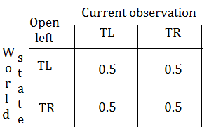
 ➁when opening the left door, below exhibits the observation probability given the world state is tiger left and right respectively.
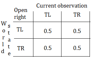
 ➂when opening the right door, below exhibits the observation probability given the world state is tiger left and right respectively.
[2]
What decision should we make?
Before we make a decision to open the correct door, we should have gathered sufficient information pertaining to the possible changes of probability distribution of tiger’s location, that’s to keep track of the belief history.
Reinforcement learning is to learn the model and planning.
Suppose the model is of no question in this example of tiger problem, we need to maintain a list of all possibilities of the belief changes, such history is build by listening in each step.
[3]
Belief update::mjtsai1974
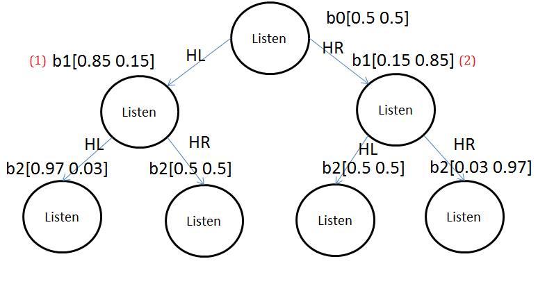
By listening in each step, we can gather information of tiger location, that’s the belief, based on history of such belief, we can then have a plan, i.e, the action to take after HL$\rightarrow$HL, HL$\rightarrow$HR.
-
Begin from initial point
We are given the tiger is at left and right with each probability $50%$ respectively, that’s $b_{0}\lbrack 0.5\;0.5\rbrack$, the first $0.5$ is the probability for tiger at left side, the similarity for tiger at the right side.
-
From init$\rightarrow$HL
Given that you are hearning tiger left, we’d like to calculate the belief at this moment.
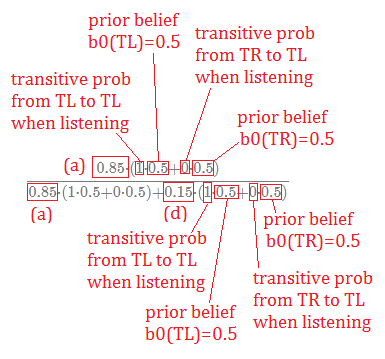
➀$b_{1}(TL)$
=$P(TL\vert HL,listen,b_{0})$
=$\frac {P(HL\vert TL,listen,b_{0})\cdot P(TL\vert listen,b_{0})}{P(HL\vert listen,b_{0})}$
=$\frac {P(HL\vert TL,listen,b_{0})\cdot\sum_{S}P(TL\vert listen,S)\cdot b_{0}(S)}{\sum_{S^{''}}P(HL\vert listen,S^{''})\cdot\sum_{S^{'}}P(S^{''}\vert listen,S^{'})\cdot b_{0}(S^{'})}$
=$\frac {0.85\cdot(1\cdot 0.5+0\cdot 0.5)}{0.85\cdot(1\cdot 0.5+0\cdot 0.5)+0.15\cdot(1\cdot 0.5+0\cdot 0.5)}$
=$0.85$
$\Rightarrow$We are now asking for belief state of tiger left, given that we are hearing left, thus the likeli should be the probability that we hear tiger left given that tiger is left, multiply by probability of tiger left, given from the prior belief state of tiger left(and by listen), divided by the total probability that we make the observation of hearing tiger left.
$\Rightarrow$The total probability of hearing tiger left is summing over all states($S^{''}$), the probability of hearing tiger left given that the tiger state is $S^{''}$, in turn multiply by summing over the state $S^{'}$, the transitive probabilities from $S^{'}$ to $S^{''}$ by listening, finally multiply with the prior belief, the probability that the world state is $S^{'}$.
 ➁$b_{1}(TR)$
=$P(TR\vert HR,listen,b_{0})$
=$\frac {P(HR\vert TR,listen,b_{0})\cdot P(TR\vert listen,b_{0})}{P(HR\vert listen,b_{0})}$
=$\frac {P(HR\vert TR,listen,b_{0})\cdot\sum_{S}P(TR\vert listen,S)\cdot b_{0}(S)}{\sum_{S^{''}}P(HR\vert listen,S^{''})\cdot\sum_{S^{'}}P(S^{''}\vert listen,S^{'})\cdot b_{0}(S^{'})}$
=$\frac {0.15\cdot(0\cdot 0.5+1\cdot 0.5)}{0.15\cdot(0\cdot 0.5+1\cdot 0.5)+0.85\cdot(0\cdot 0.5+1\cdot 0.5)}$
=$0.15$
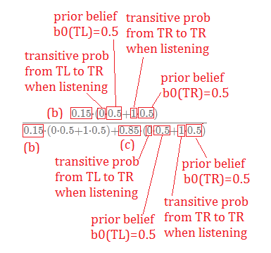 $\Rightarrow$we have belief updated from $b_{0}$ to $b_{1}\lbrack 0.85\;0.15\rbrack$ in this brach.
-
From init$\rightarrow$HR
Given that you are hearning tiger right, we’d like to calculate the belief at this moment.
➀$b_{1}(TL)$
=$P(TL\vert HL,listen,b_{0})$
=$\frac {0.15\cdot(1\cdot 0.5+0\cdot 0.5)}{0.15\cdot(1\cdot 0.5+0\cdot 0.5)+0.85\cdot(1\cdot 0.5+0\cdot 0.5)}$
=$0.15$
➁$b_{1}(TR)$
=$P(TR\vert HR,listen,b_{0})$
=$\frac {0.85\cdot(0\cdot 0.5+1\cdot 0.5)}{0.85\cdot(0\cdot 0.5+1\cdot 0.5)+0.1\cdot(0\cdot 0.5+1\cdot 0.5)}$
=$0.85$
$\Rightarrow$we have belief updated from $b_{0}$ to $b_{1}\lbrack 0.15\;0.85\rbrack$ in this brach.
-
From init$\rightarrow$HL$\rightarrow$HL
Suppose that you are hearning tiger left after hearing tiger left, we’d like to calculate the belief at this moment.
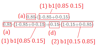
➀$b_{2}(TL)$
=$P(TL\vert HL,listen,b_{1})$
=$\frac {0.85\cdot(1\cdot 0.85+0\cdot 0.15)}{0.85\cdot(1\cdot 0.85+0\cdot 0.15)+0.15\cdot(1\cdot 0.15+0\cdot 0.85)}$
=$0.967986$
$\approx 0.97$
 ➁$b_{2}(TR)$
=$P(TR\vert HR,listen,b_{1})$
=$\frac {0.15\cdot(0\cdot 0.85+1\cdot 0.15)}{0.15\cdot(0\cdot 0.85+1\cdot 0.15)+0.85\cdot(0\cdot 0.15+1\cdot 0.85)}$
=$0.03020$
$\approx 0.03$
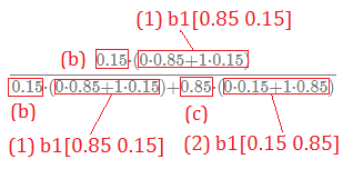 $\Rightarrow$we have belief updated from $b_{1}\lbrack 0.85\;0.15\rbrack$ to $b_{2}\lbrack 0.97\;0.03\rbrack$ in this brach.
-
From init$\rightarrow$HL$\rightarrow$HR
Suppose that you are hearning tiger left after hearing tiger right, we’d like to calculate the belief at this moment.
➀$b_{2}(TL)$
=$P(TL\vert HL,listen,b_{1})$
=$\frac {0.15\cdot(1\cdot 0.85+0\cdot 0.15)}{0.15\cdot(1\cdot 0.85+0\cdot 0.15)+0.85\cdot(1\cdot 0.15+0\cdot 0.85)}$
=$0.5$
➁$b_{2}(TR)$
=$P(TR\vert HR,listen,b_{1})$
=$\frac {0.85\cdot(0\cdot 0.85+1\cdot 0.15)}{0.85\cdot(0\cdot 0.85+1\cdot 0.15)+0.15\cdot(0\cdot 0.15+1\cdot 0.85)}$
=$0.5$
$\Rightarrow$we have belief updated from $b_{1}\lbrack 0.85\;0.15\rbrack$ to $b_{2}\lbrack 0.5\;0.5\rbrack$ in this brach.
Notes::mjtsai1974
The likeli in the nominator is goint to use the belief distribution at the node which it is branching from as the prior.
-
From init$\rightarrow$HR$\rightarrow$HL
Suppose that you are hearning tiger left after hearing tiger right, we’d like to calculate the belief at this moment.
➀$b_{2}(TL)$
=$P(TL\vert HL,listen,b_{1})$
=$\frac {0.85\cdot(1\cdot 0.15+0\cdot 0.85)}{0.85\cdot(1\cdot 0.15+0\cdot 0.85)+0.15\cdot(1\cdot 0.85+0\cdot 0.15)}$
=$0.5$
➁$b_{2}(TR)$
=$P(TR\vert HR,listen,b_{1})$
=$\frac {0.15\cdot(0\cdot 0.15+1\cdot 0.85)}{0.15\cdot(0\cdot 0.15+1\cdot 0.85)+0.85\cdot(0\cdot 0.85+1\cdot 0.15)}$
$0.5$
$\Rightarrow$we have belief updated from $b_{1}\lbrack 0.15\;0.85\rbrack$ to $b_{2}\lbrack 0.5\;0.5\rbrack$ in this brach.
-
From init$\rightarrow$HR$\rightarrow$HR
Suppose that you are hearning tiger right after hearing tiger right, we’d like to calculate the belief at this moment.
➀$b_{2}(TL)$
=$P(TL\vert HL,listen,b_{1})$
=$\frac {0.15\cdot(1\cdot 0.15+0\cdot 0.85)}{0.15\cdot(1\cdot 0.15+0\cdot 0.85)+0.85\cdot(1\cdot 0.85+0\cdot 0.15)}$
$\approx 0.03$
➁$b_{2}(TR)$
=$P(TR\vert HR,listen,b_{1})$
=$\frac {0.85\cdot(0\cdot 0.15+1\cdot 0.85)}{0.85\cdot(0\cdot 0.15+1\cdot 0.85)+0.15\cdot(0\cdot 0.85+1\cdot 0.15)}$
=$\approx 0.97$
$\Rightarrow$we have belief updated from $b_{1}\lbrack 0.15\;0.85\rbrack$ to $b_{2}\lbrack 0.03\;0.97\rbrack$ in this brach.
[4]
Have a tea break before opening the door
Making belief update over theses steps, we can do some plan on the belief histroy, if we make continuous 2 observations of hearing tiger left, the belief would be the probability distribution over tiger left and tiger right, which is $b_{2}\lbrack 0.97\;0.03\rbrack$. Should we open the right door??
The ideal answer would be discusssed in my next article.
[5]
Make extra one step
-
From init$\rightarrow$HL$\rightarrow$HL$\rightarrow$HL
Guess what, if we keep on following in this path, from init to hearning tiger left, next to hearing tiger left, next to hearing tiger left, we’d like to make the belief update at this moment.
➀$b_{3}(TL)$
=$P(TL\vert HL,listen,b_{2})$
=$\frac {0.85\cdot\lbrack(1\cdot 0.97+0\cdot 0.03)+(1\cdot 0.5+0\cdot 0.5)\rbrack}{0.85\cdot\lbrack(1\cdot 0.97+0\cdot 0.03)+(1\cdot 0.5+0\cdot 0.5)\rbrack+0.15\cdot\lbrack(1\cdot 0.5+0\cdot 0.5)+(1\cdot 0.03+0\cdot 0.97)\rbrack}$
$\approx 0.94$
 ➁$b_{3}(TR)$
=$P(TR\vert HR,listen,b_{2})$
=$\frac {0.15\cdot\lbrack(0\cdot 0.97+1\cdot 0.03)+(0\cdot 0.5+1\cdot 0.5)\rbrack}{0.15\cdot\lbrack(0\cdot 0.97+1\cdot 0.03)+(0\cdot 0.5+1\cdot 0.5)\rbrack+0.85\cdot\lbrack(0\cdot 0.5+1\cdot 0.5)+(0\cdot 0.03+1\cdot 0.97)\rbrack}$
$\approx 0.06$
$\Rightarrow$we have belief updated from $b_{2}\lbrack 0.97\;0.03\rbrack$ to $b_{3}\lbrack 0.94\;0.06\rbrack$ in this brach.

-
From init$\rightarrow$HL$\rightarrow$HL$\rightarrow$HR
Go from init to hearning tiger left, next to hearing tiger left, next to hearing tiger right, we’d like to make the belief update at this moment.
➀$b_{3}(TL)$
=$P(TL\vert HL,listen,b_{2})$
=$\frac {0.15\cdot\lbrack(1\cdot 0.97+0\cdot 0.03)+(1\cdot 0.5+0\cdot 0.5)+(1\cdot 0.03+0\cdot 0.97)\rbrack}{0.15\cdot\lbrack(1\cdot 0.97+0\cdot 0.03)+(1\cdot 0.5+0\cdot 0.5)+(1\cdot 0.03+0\cdot 0.97)\rbrack+0.85\cdot(1\cdot 0.5+0\cdot 0.5)}$
=$0.3463$
 ➁$b_{3}(TR)$
=$P(TR\vert HR,listen,b_{2})$
=$\frac {0.85\cdot\lbrack(0\cdot 0.97+1\cdot 0.03)+(0\cdot 0.5+1\cdot 0.5)+(0\cdot 0.03+1\cdot 0.97)\rbrack}{0.85\cdot\lbrack(0\cdot 0.97+1\cdot 0.03)+(0\cdot 0.5+1\cdot 0.5)+(0\cdot 0.03+1\cdot 0.97)\rbrack+0.15\cdot(0\cdot 0.5+1\cdot 0.5)}$
=$0.9444$
 $\Rightarrow$The $b_{3}(TL)$+$b_{3}(TR)$ not equal to $1$, we are encounter a big problem, guess what? By normalization, we can get the correct answer.
➂$N(b_{3}(TL))$=$\frac {0.3463}{0.3463+0.9444}$=$0.268217$
➃$N(b_{3}(TR))$=$\frac {0.9444}{0.3463+0.9444}$=$0.73169$
$\Rightarrow$we have belief updated from $b_{2}\lbrack 0.97\;0.03\rbrack$ to $b_{3}\lbrack 0.27\;0.73\rbrack$ in this brach.
-
From init$\rightarrow$HL$\rightarrow$HR$\rightarrow$HL
Go from init to hearning tiger left, next to hearing tiger right, next to hearing tiger left, we’d like to make the belief update at this moment.
➀$b_{3}(TL)$
=$P(TL\vert HL,listen,b_{2})$
=$\frac {0.85\cdot\lbrack(1\cdot 0.5+0\cdot 0.5)+(1\cdot 0.97+0\cdot 0.03)+(1\cdot 0.5+0\cdot 0.5)\rbrack}{0.85\cdot\lbrack(1\cdot 0.5+0\cdot 0.5)+(1\cdot 0.97+0\cdot 0.03)+(1\cdot 0.5+0\cdot 0.5)\rbrack+0.15\cdot(1\cdot 0.03+0\cdot 0.97)}$
$\approx 0.997$
➁$b_{3}(TR)$
=$P(TR\vert HR,listen,b_{2})$
=$\frac {0.15\cdot\lbrack(0\cdot 0.5+1\cdot 0.5)+(0\cdot 0.97+1\cdot 0.03)+(0\cdot 0.5+1\cdot 0.5)\rbrack}{0.15\cdot\lbrack(0\cdot 0.5+1\cdot 0.5)+(0\cdot 0.97+1\cdot 0.03)+(0\cdot 0.5+1\cdot 0.5)\rbrack+0.85\cdot(0\cdot 0.03+1\cdot 0.97)}$
$\approx 0.158$
➂$N(b_{3}(TL))$=$\frac {0.997}{0.997+0.158}$=$0.863$
➃$N(b_{3}(TR))$=$\frac {0.158}{0.997+0.158}$=$0.137$
$\Rightarrow$we have belief updated from $b_{2}\lbrack 0.5\;0.5\rbrack$ to $b_{3}\lbrack 0.86\;0.14\rbrack$ in this brach.
-
From init$\rightarrow$HL$\rightarrow$HR$\rightarrow$HR
Go from init to hearning tiger left, next to hearing tiger right, next to hearing tiger right, we’d like to make the belief update at this moment.
➀$b_{3}(TL)$
=$P(TL\vert HL,listen,b_{2})$
=$\frac {0.15\cdot\lbrack(1\cdot 0.5+0\cdot 0.5)+(1\cdot 0.03+0\cdot 0.97)\rbrack}{0.15\cdot\lbrack(1\cdot 0.5+0\cdot 0.5)+(1\cdot 0.03+0\cdot 0.97)\rbrack+0.85\cdot\lbrack(1\cdot 0.97+0\cdot 0.03)+(1\cdot 0.5+0\cdot 0.5)\rbrack}$
=$0.0598194131$
$\approx 0.06$
➁$b_{3}(TR)$
=$P(TR\vert HR,listen,b_{2})$
=$\frac {0.85\cdot\lbrack(0\cdot 0.5+1\cdot 0.5)+(0\cdot 0.03+1\cdot 0.97)\rbrack}{0.85\cdot\lbrack(0\cdot 0.5+1\cdot 0.5)+(0\cdot 0.03+1\cdot 0.97)\rbrack+0.15\cdot\lbrack(0\cdot 0.97+1\cdot 0.03)+(0\cdot 0.5+1\cdot 0.5)\rbrack}$
=$0.94$
$\Rightarrow$we have belief updated from $b_{2}\lbrack 0.5\;0.5\rbrack$ to $b_{3}\lbrack 0.06\;0.94\rbrack$ in this brach.
-
From init$\rightarrow$HR$\rightarrow$HL$\rightarrow$HL
Go from init to hearning tiger right, next to hearing tiger left, next to hearing tiger left, we’d like to make the belief update at this moment.
➀$b_{3}(TL)$
=$P(TL\vert HL,listen,b_{2})$
=$\frac {0.85\cdot\lbrack(1\cdot 0.5+0\cdot 0.5)+(1\cdot 0.97+0\cdot 0.03)\rbrack}{0.85\cdot\lbrack(1\cdot 0.5+0\cdot 0.5)+(1\cdot 0.97+0\cdot 0.03)\rbrack+0.15\cdot\lbrack(1\cdot 0.5+0\cdot 0.5)+(1\cdot 0.03+0\cdot 0.97)\rbrack}$
$\approx 0.94$
➁$b_{3}(TR)$
=$P(TR\vert HR,listen,b_{2})$
=$\frac {0.15\cdot\lbrack(0\cdot 0.5+1\cdot 0.5)+(0\cdot 0.97+1\cdot 0.03)\rbrack}{0.15\cdot\lbrack(0\cdot 0.5+1\cdot 0.5)+(0\cdot 0.97+1\cdot 0.03)\rbrack+0.85\cdot\lbrack(0\cdot 0.5+1\cdot 0.5)+(0\cdot 0.03+1\cdot 0.97)\rbrack}$
$\approx 0.06$
$\Rightarrow$we have belief updated from $b_{2}\lbrack 0.5\;0.5\rbrack$ to $b_{3}\lbrack 0.94\;0.06\rbrack$ in this brach.
-
From init$\rightarrow$HR$\rightarrow$HL$\rightarrow$HR
➀$b_{3}(TL)$
=$P(TL\vert HL,listen,b_{2})$
=$\frac {0.15\cdot\lbrack(1\cdot 0.5+0\cdot 0.5)+(1\cdot 0.5+0\cdot 0.5)+(1\cdot 0.03+0\cdot 0.97)\rbrack}{0.15\cdot\lbrack(1\cdot 0.5+0\cdot 0.5)+(1\cdot 0.5+0\cdot 0.5)+(1\cdot 0.03+0\cdot 0.97)\rbrack+0.85\cdot\lbrack(1\cdot 0.97+0\cdot 0.03)+(1\cdot 0.5+0\cdot 0.5)\rbrack}$
$\approx 0.11$
➁$b_{3}(TR)$
=$P(TR\vert HR,listen,b_{2})$
=$\frac {0.85\cdot\lbrack(0\cdot 0.5+1\cdot 0.5)+(0\cdot 0.5+1\cdot 0.5)+(0\cdot 0.03+1\cdot 0.97)\rbrack}{0.85\cdot\lbrack(0\cdot 0.5+1\cdot 0.5)+(0\cdot 0.5+1\cdot 0.5)+(0\cdot 0.03+1\cdot 0.97)\rbrack+0.15\cdot(0\cdot 0.97+1\cdot 0.03)}$
$\approx 0.9913$
➂$N(b_{3}(TL))$=$\frac {0.11}{0.11+0.9913}$=$0.099\approx 0.1$
➃$N(b_{3}(TR))$=$\frac {0.9913}{0.11+0.9913}$=$0.9$
$\Rightarrow$we have belief updated from $b_{2}\lbrack 0.5\;0.5\rbrack$ to $b_{3}\lbrack 0.1\;0.9\rbrack$ in this brach.
-
From init$\rightarrow$HR$\rightarrow$HR$\rightarrow$HL
➀$b_{3}(TL)$
=$P(TL\vert HL,listen,b_{2})$
=$\frac {0.85\cdot\lbrack(1\cdot 0.03+0\cdot 0.97)+(1\cdot 0.5+0\cdot 0.5)+(1\cdot 0.97+0\cdot 0.03)\rbrack}{0.85\cdot\lbrack(1\cdot 0.03+0\cdot 0.97)+(1\cdot 0.5+0\cdot 0.5)+(1\cdot 0.97+0\cdot 0.03)\rbrack+0.15\cdot(1\cdot 0.5+0\cdot 0.5)}$
$\approx 0.9444$
➁$b_{3}(TR)$
=$P(TR\vert HR,listen,b_{2})$
=$\frac {0.15\cdot\lbrack(0\cdot 0.97+1\cdot 0.03)+(0\cdot 0.5+1\cdot 0.5)+(0\cdot 0.03+1\cdot 0.97)\rbrack}{0.15\cdot\lbrack(0\cdot 0.97+1\cdot 0.03)+(0\cdot 0.5+1\cdot 0.5)+(0\cdot 0.03+1\cdot 0.97)\rbrack+0.85\cdot(0\cdot 0.5+1\cdot 0.5)}$
$\approx 0.3461538$
➂$N(b_{3}(TL))$=$\frac {0.9444}{0.94444+0.3461538}$=$0.7317\approx 0.73$
➃$N(b_{3}(TR))$=$\frac {0.3461538}{0.94444+0.3461538}$=$0.268221\approx 0.27$
$\Rightarrow$we have belief updated from $b_{2}\lbrack 0.03\;0.97\rbrack$ to $b_{3}\lbrack 0.73\;0.27\rbrack$ in this brach.
-
From init$\rightarrow$HR$\rightarrow$HR$\rightarrow$HR
➀$b_{3}(TL)$
=$P(TL\vert HL,listen,b_{2})$
=$\frac {0.15\cdot\lbrack(1\cdot 0.03+0\cdot 0.97)+(1\cdot 0.5+0\cdot 0.5)\rbrack}{0.15\cdot\lbrack(1\cdot 0.03+0\cdot 0.97)+(1\cdot 0.5+0\cdot 0.5)\rbrack+0.85\cdot\lbrack(1\cdot 0.97+0\cdot 0.03)+(1\cdot 0.5+0\cdot 0.5)\rbrack}$
=$0.0598$
$\approx 0.06$
➁$b_{3}(TR)$
=$P(TR\vert HR,listen,b_{2})$
=$\frac {0.85\cdot\lbrack(0\cdot 0.03+1\cdot 0.97)+(0\cdot 0.5+1\cdot 0.5)\rbrack}{0.85\cdot\lbrack(0\cdot 0.03+1\cdot 0.97)+(0\cdot 0.5+1\cdot 0.5)\rbrack+0.15\cdot\lbrack(0\cdot 0.97+1\cdot 0.03)+(0\cdot 0.5+1\cdot 0.5)\rbrack}$
=$0.9401$
$\approx 0.94$
$\Rightarrow$we have belief updated from $b_{2}\lbrack 0.03\;0.97\rbrack$ to $b_{3}\lbrack 0.06\;0.94\rbrack$ in this brach.
Belief Space
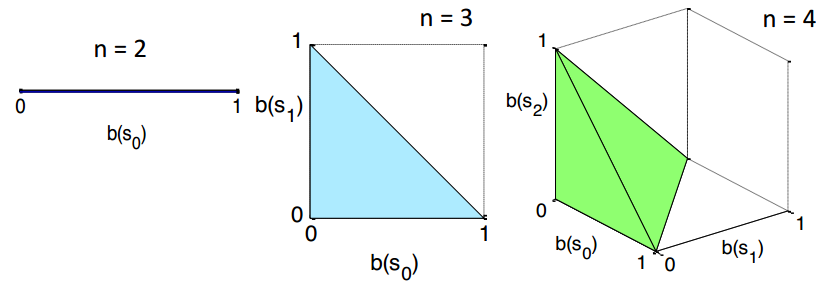
Belief is a probability distribution over states.
➀$\sum_{S}b(S)$=$1$
➁for $n$ states, belief has $n-1$ degree of freedom
➂belief lives in a $n-1$ dimensional simplex, i.e, a world of 2 states, $b(S_{0})$ is determined by the value of $b(S_{1})$, it has 1 degree of freedom. i.e, a world of 3 states, $b(S_{i})$ is determined by the other 2 values, it has 2 degree of freedom.
Addendum
➀Partial Observable Markov Decision Process, Charles IsBell, Michael Littman, Reinforcement Learning By Georgia Tech(CS8803)
➁Decsision Making in Intellingent Systems: POMDP, 14 April 2008, Frans Oliehoek
➂Intro to POMDPs, CompSci 590.2 Reinforcement Learning
21 Jul 2020
Prologue To Partial Observable Markov Decision Process - Part 1
This post is an entry of POMDP(Partial Observable Markov Decision Process), from the most foundamental to the belief update.
Summary Of All Markov Models
[1]
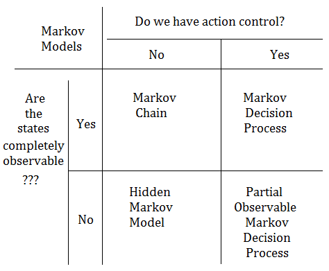
Markov chain
➀finite number of discrete states with probabilistic transition between states.
➁the Makrov property is that next state is determined by current state only!!
[2]
Hidden Markov model
➀all the same in Markov chain, except that we're unsure which state we are in.
➁the current state emits an observation.
[3]
Markov decision process
➀finite number of discrete states.
➁probabilistic transition between states and executable actions in each state.
➂next state is determined by current state and current action.
➃the execution of an action might lead to unexpected result due to random stochasticity.
[4]
Partial observal Markov decision process
➀all the same as Markov decision process, except that we're unsure which state we are in.
➁the current state emits an observation.
Below table exhibits the summary:
Belief State In POMDP
Below exhibits the POMDP model, wherein the probability distribution is over the world states with true state is only partially observable.
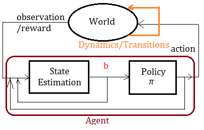
➀the agent keeps/maintains an internal belief state, say $b$, that summarizes its experience.
➁the agent makes state estimation to update from belief state $b$ to next belief state $b^{'}$, based on the last action it has taken, the current observation it has made, and the previous belief state $b$.
[Question]Why Belief State in POMDP?
[Answer]
➀the state of the real world is only partially observable.
➁the agent needs to learn how the observations might aid its performance.
➂there might exists no immediate observation pertaining to the desired state.
$\Rightarrow$This rerveals that the states are probabilistically distributed over the given observations at any time, such probability distribution varies over time, that’s why we have belief state from initial $b$ to $b^{'}$, or say from $b_{0}$ to $b_{1}$, $b_{2}$,…,$b_{i}$, $b_{i+1}$,…,$b_{\infty}$.
➃the whole POMDP is illustrated/iterated in the environment of uncertainty.
➄uncertainty about action outcome, about the world state due to imperfect(partial) information.
POMDP Parameters
➀initial belief:
$b(S)$=$P(S)$, this means the probability for we are in state $S$.
➁belief state updating:
$b^{'}(S^{'})$=$P(S^{'}|O,A,b)$, this represents the probability for we are in state $S^{'}$, given that we take action $A$, make observation $O$, from previous belief state distribution, say $b$.
➂observation function:
$\Omega(S^{'},A,O)$=$P(O|S^{'},A)$, it represents the probability for we make observation $O$, given that we are transiting to state $S^{'}$, by taking action $A$.
➃transitive probability:
$T(S,A,S^{'})$=$P(S^{'}|S,A)$, it represents the probability for we transit from $S$ to $S^{'}$, by taking action $A$.
➄rewards:
$R(A,b)$=$\sum_{S}R(S,A)\cdot b(S)$, where $R(S,A)$ is the same as it is in MDP, and the reward is summing over the reward by taking action $A$ with proportion to the probabilistic distribution for each state $S$ in $b$.
Understand The Belief State $b$
Suppose we are given $n$ underlying states, a discrete state space of size $n$, then the belief state $b$ is a vector of $n$ states.
Partial observable turns discrete problem of $n$ states into continuous problem, a POMDP with $n$ states induces an $n$-dimensional belief-MDP.
[Answer]
The true state is only partial observable, where $b(S)$=probability of being in state $S$.
At each step, the agent:
➀takes some action, say $A$
➁transites to next state $S^{'}$ form state $S$
➂makes observation $O$, with probability $P(O|S^{'},A)$
➃suppose we are given initial belief state $b$, after ➀,➁,➂, the probabilistic distribution over the belief state would definitely be changed.
-
The posterior belief
That’s why we need to make belief update, say the posterior belief:
$b^{'}(S^{'})$=$\alpha\cdot P(O|S^{'},A)\cdot\sum_{S}P(S^{'}|S,A)\cdot b(S)$
, where $\alpha$ is certain coefficient, such belief update is continuous rather than discrete!!!
-
Continuous belief update
POMDP could be regarded as continuous belief update over underlying MDP states, as the agent’s belief is encoded through a continuous belief state.
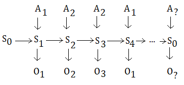 Each MDP state is a probability distribution(continuous belief state) over the state of the original POMDP.
POMDP: Belief Update
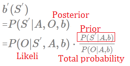
$b^{'}(S^{'})$
=$P(S^{'}|A,O,b)$, we believe we are in state $S^{'}$, given observation $O$
=$P(O|S^{'},A,b)\cdot\frac {P(S^{'}|A,b)}{P(O|A,b)}$
mjtsai think we can treat $b'(S')$ as $P(S'|O)$ in viewpoint of Bayer theorem.
-
$P(O|S^{'},A,b)$
➀it is the probability that we make observation $O$, given that we are in state $S^{'}$, by taking action $A$, probabilistically distributed over belief state $b$(or say from previous belief state $b$).
➁therefore, we can treat $P(O|S^{'},A,b)$=$P(O|S^{'})$
-
$P(S^{'}|A,b)$
This stands for the probability that we are in $S^{'}$, given action $A$ has been taken, from belief state $b$
, where $P(S^{'}|A,b)$=$\sum_{S}P(S^{'}|A,S)\cdot b(S)$ and this $b$ is to be believed a vector of states, a vector of state space.
-
$P(O|A,b)$
This indicates we make observation $O$, given that we has taken action $A$, from belief state $b$
, this is a normalization factor, where
$P(O|A,b)$
=$\sum_{S^{''}}P(O|S^{''})\cdot P(S^{''}|A,b)$
=$\sum_{S^{''}}P(O|S^{''})\cdot\sum_{S}P(S^{''}|A,S)\cdot b(S)$
Notes::mjtsai1974
This expression is asking for the probability of the fact that we are in state $S^{'}$, given that we make observation $O$, by taking action $A$, from somewhat belief state $b$.
It could be further expanded as the qualitative probability that we make observation $O$, given that we are in state $S^{'}$, by taking action $A$, from belief state $b$. Such likeli in turn multiplied by the probabilty, which is a prior that we are in $S^{'}$, by taking action $A$, from belief state $b$. Finally, over the total/marginal probability probability that we make observation $O$, given that we take action $A$, from somewhat belief state $b$.
Addendum
➀Partial Observable Markov Decision Process, Charles IsBell, Michael Littman, Reinforcement Learning By Georgia Tech(CS8803)
➁Partially Observable Markov Decision Process, Geoff Hollinger, 2007 fall
➂Prof. Dr.-Ing. Stefan Kopp, 2010, Bielefed University
22 Apr 2020
Prologue To Model-Based RL Algorithm RMAX - Part 5
This article reviews RMAX in summary of illustration.
Two Main Reinforcement Learning Approaches: Recap
[1]
Model-free approachs
They don’t learn a model, model-free approachs learn value function or policy function directly, that is to say they directly estimate state-action value function.
-
Q learning
$Q_{T+1}(S,A)$=$R_{T}(S,A,S^{'})$+$\gamma\cdot max_{A^{'}}Q_{T}(S^{'},A^{'})$
$\Rightarrow Q_{T+1}^{\ast}(S,A)$=$(1-\alpha)\cdot Q_{T}(S,A)$+$\alpha\cdot Q_{T+1}(S,A)$
-
Temporal difference in value function form(without action)
[The rule]
Eposide $T$:
$\;\;$For all $S$, $e(S)$=$0$ at start of eposide, $V_{T}(S)$=$V_{T-1}(S)$
$\;\;$After $S_{t-1}\xrightarrow{r_{t}}S_{t}$:(from step $t-1$ to $t$ with reward $r_{t}$)
$\;\;\;e(S_{t-1})$=$e(S_{t-1})$+$1$:
$\;\;\;\;$Update eligibility of $S_{t-1}$ after arriving to $S_{t}$
$\;\;$For all $S$,
$\;\;V_{T}(S)$=$V_{T-1}(S)$+$\alpha_{T}\cdot(r_{t}+\gamma\cdot V_{T-1}(S_{t})-V_{T-1}(S_{t-1}))$
$\;\;\;e(S_{t-1})$=$\lambda\cdot\gamma\cdot e(S_{t-1})$:
$\;\;\;\;$before transite from $S_{t-1}$ to $S_{t}$ in next iteration
- Temporal difference in Q form(with action)
➀the Q function takes state and action as input parameters.
$Q^{\pi}(S_{t},A_{t})$=$E\lbrack R_{t+1}+\gamma\cdot R_{t+2}+\gamma^{2}\cdot R_{t+3}+…\vert S_{t},A_{t}\rbrack$
➂take action $A$ to transite from state $S$ to $S’$
$Q_{T}(S,A)$
=$Q_{T-1}(S,A)$+$\alpha_{T}\cdot(R(S,A)$+$\gamma\cdot max_{A’}Q_{T-1}(S’,A’)$-$Q_{T-1}(S,A))$
By repeating above Bellman equation in Q form, the Q value will finally get converged, usually denoted as $Q^{*}(S,A)$, and it’s the policy for you to take action $A$ when you are in state $S$ to get the maximum value.
[2]
Model-base approachs
Given sample of data seen so far:
➀build the explicit model of MDP and compute policy for it in the beginning.
➁explore the environment in the given data, learn the transitive probability $P(S,A,S^{'})$ and reward function $R(S,A)$ in accordance to state-action pair.
➂repeat until the transitive probability $P(S,A,S^{'})$ and reward function $R(S,A)$ is to be believed converged to an acceptable confidence interval, during the convergence period, recompute the policy for that state once the transitive probability and reward function has been updated.
One of such approaches is the RMAX algorithm.
RMAX Algorithm Summary
[1]
Proceed with explore or exploit
By the given sample of data, this algorithm proceeds with explore to some unknown states or exploit over the same state, and you will never know you are exploring or exploting.
[2]
Implicit explore or exploit lemma
After every $T$ steps, you either:
➀achieves or attains the near optimal reward for these $T$ steps.
➁explore to certain unknown state in high probability, learns a little about an unknown state.
[3]
The RMAX algorithm
-
Initialization
➀add the state $S_{0}$ to the MDP model
➁set $P(S_{0},A,S)$=$1$ for all state $S$
➂set $R(S,A)$=$R_{max}$ for all state $S$ and action $A$
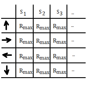 ➃set all states to unknown states, excepts for $S_{0}$
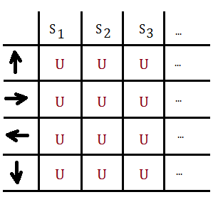 ➄set all visited counter of state-action pairs to $0$
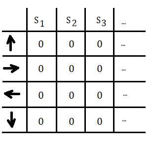
-
Repeat
➀compute a $T$-step policy for current state $S$ and execute it
➁for any visited state-action pair, keep track of its count and reward with respect to state transition from $S$ to $S^{'}$
➂if the same state-action pair has been visited over enough times to estimate $P(S,A,S^{'})$ and $R(S,A)$, update the transitive probability, turn the state-action pair from unknown to know, and repeat from ➀
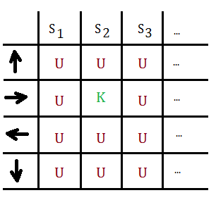
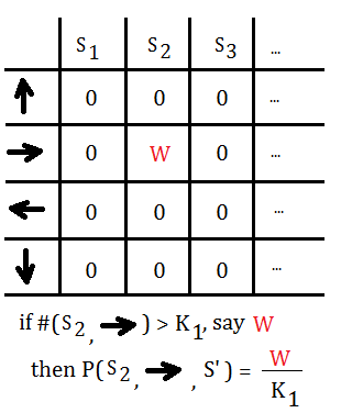 ➃loops through ➀,➁,➃ until all states has become known
[4]
How many times are enough?
- By Chernoff Bounds For Bernoulli Random Variable
We have $P(\sum_{i=1}^{n}Z_{i}>a)<e^{-\frac {a^{2}}{2\cdot n}}$, where $Z_{1}$,$Z_{2}$,…,$Z_{n}$ are the $n$ distinct independent trials on state $G_{i}$, and $a$ is the error term, such inequality bounds the error probability by $e^{-\frac {a^{2}}{2\cdot n}}$ that after $n$ independent trials on state $G_{i}$, the total estimate bias is greater than the error term $a$.
[5]
Put it all together
With probability at least $1-\delta$, the RMAX algorithm will reach $\varepsilon$ close to optimal policy, in time polinomial in the number of states, the number of actions, $\frac {1}{\delta}$, $\frac {1}{\varepsilon}$.
- Every $T$ steps
By implicit explore or exploit lemma:
➀achieve near optimal reward, or
➁explore to certain unknown state with high probability. Since the number of states and actions are finite, it wouldn’t take too long before all states turn into known!
Addendum
➀R-max: A General Polynomial Time Algorithm for Near-Optimal Reinforcement Learning, Ronen I. Brafman, CS in Ben-Gurion University, Moshe Tennenholtz, CS in Stanford University
➁Reinforcement Learning: Machine Learning - CSE446, Carlos Guestrin, University of Washington, June 5, 2013


 Suppose we begin from root node of certain action $A$, with probabilitistic distribution over observations $\{O_{1},O_{2},…,O_{K}\}$, and totally $H$ steps to go.
 $V_{P_{t}(a_{i})}(b)$=$\sum_{s}R(s,a_{i})\cdot b(s)$, for $s\in\{s_{0},s_{1}\}$, given that $b_{0}\lbrack 0.5\;0.5\rbrack$, and immediate rewards are initialized as shown, then


 ➁combine these linear lines together we get:
 ➂by pruning and partioning we can get the optimal actions in each region:
 ➃we next extend from $a_{2}$ at $t$=$2$, suppose we get optimal action of region partitioned in below:
 ➄put it all together, we could get the optimal actions as a whole image:

 ➁we then start from the path of $1$-st action $a_{2}$, make observation $o_{1}$, then $2$-nd action $a_{2}$, for simplicity, we get below optimal actions in each region:
 ➂we next start from the path of $1$-st action $a_{2}$, make observation $o_{3}$, then $2$-nd action $a_{1}$, for simplicity, we get below optimal actions in each region:
 ➃put it together, we could get the optimal action partitions in below:
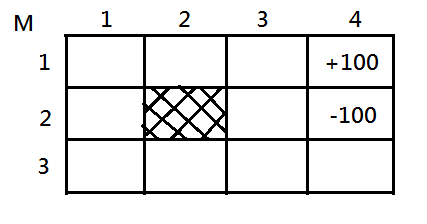 ➁
➁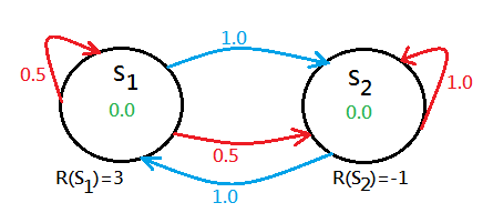
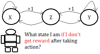
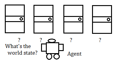 ➁the agent don’t know what state he is in if he didn’t get reward after taking action.

 ➁when you open the left door, the tiger has $50%$ to stay behind the left door, or $50%$ to stay behind the right door.


 ➁when opening the left door, below exhibits the observation probability given the world state is tiger left and right respectively.
 ➂when opening the right door, below exhibits the observation probability given the world state is tiger left and right respectively.

 ➁$b_{1}(TR)$
 $\Rightarrow$we have belief updated from $b_{0}$ to $b_{1}\lbrack 0.85\;0.15\rbrack$ in this brach.
 ➁$b_{2}(TR)$
 $\Rightarrow$we have belief updated from $b_{1}\lbrack 0.85\;0.15\rbrack$ to $b_{2}\lbrack 0.97\;0.03\rbrack$ in this brach.
 ➁$b_{3}(TR)$
 ➁$b_{3}(TR)$
 $\Rightarrow$The $b_{3}(TL)$+$b_{3}(TR)$ not equal to $1$, we are encounter a big problem, guess what? By normalization, we can get the correct answer.


 Each MDP state is a probability distribution(continuous belief state) over the state of the original POMDP.
 ➃set all states to unknown states, excepts for $S_{0}$
 ➄set all visited counter of state-action pairs to $0$

 ➃loops through ➀,➁,➃ until all states has become known