Model-Based RL Algorithm RMAX - Part 4

26 Mar 2020

Prologue To Model-Based RL Algorithm RMAX - Part 4

The RMAX theorem guarantees that the learning efficiency is polynomial and would be proved in this article.

The RMAX Theorem

[Theorem of optimality and convergence]

Given below condition:
➀let $M$ be the stochastic game with $N$ states and $k$ actions.
➁let $0 < \delta < 1$ and $\varepsilon > 0$ be constants, where $\delta$ is the error probability and $\varepsilon$ is the error term.
➂denote the policy for $M$ whose $\varepsilon$-return mixing time is $T$ by $\prod_{M}(\varepsilon,T)$.
➃denote the optimal expected return by such policy by $Opt(\prod_{M}(\varepsilon,T))$.

Then, with probability of no less than $1-\delta$ the RMAX algorithm will attain an expected return of $Opt(\prod_{M}(\varepsilon,T))-2\cdot\varepsilon$, within a number of steps polynomial in $N$,$k$,$T$,$\frac {1}{\varepsilon}$ and $\frac {1}{\delta}$.

Notes::mjtsai1974

Why the execution of the RMAX algorithm will attain an expected return of $Opt(\prod_{M}(\varepsilon,T))-2\cdot\varepsilon$?

As a result of the fact that the optimal policy is defined on $\varepsilon$-return mixing time of $T$, the real return of the execution of the RMAX algorithm must be smaller than it, thus we choose it to be $-2\cdot\varepsilon$.

Why the RMAX algorithm is polynomial?

[1] Recap on implicit explore or exploit lemma

The implicit explore or exploit lemma guarantees that the policy generated from the simulated model $M_{L}$ onto the target model $M$ could either leads to $\alpha$ close to optimal reward or explore efficiently with hight probability of at least $\frac {\alpha}{R_{max}}$, where $M_{L}\rightarrow_{\alpha}M$ and $\alpha$=$\frac {\varepsilon}{N\cdot T\cdot R_{max}}$.

[2] Due to $\alpha$ approximation

Since $\alpha$=$\frac {\varepsilon}{N\cdot T\cdot R_{max}}$, the $T$ step phases in which we are exploring in the execution of the RMAX algorithm is polynomial in $N$,$T$,$\varepsilon$.

[3] Learn over $N$ states and $k^{2}$ actions

There are totally $N$ states(or stage games) in model $M$ with $k$ actions for the agent and the adversary, therefore, we have a polynomial number of parameters to learn, say $N$ and $k$.

[4] The probability to update the unknown information

The probability the RMAX alrorithm to turn a state from unknown to known or to update statistics information is polynomial in $\varepsilon$,$T$,$N$.

[Notes] A brief summary

Base on all of above, by sampling in a large number of times, the implicit explore or exploit lemma guarantees the least probabilistic exploration, and we can ensure that the fail rate in attaining the optimal reward is quiet small, say $\delta$.

The RMAX algorithm claims that we can get near optimal reward with probability $1-\delta$ by sampling a sufficient large number of trials over the same state, which is polynomial in $\frac {1}{\delta}$.

Watch out that each trial contains either exploration or exploitation, next to prove this theorem.

The RMAX Theorem Proof::1

[1] The accuracy in the estimate of transitive probability

First, we’d like to prove that the estimate of transitive probability in the implicit explore or exploit is accurate.

The majority focus on the number of trials in this same state, that is how many times of state transition in this same state for explore or exploit could we believe that the estimated transitive probability is accurate?

[2] By sampling in a large number of trials over the same state

How many number of trials on $G_{i}$(in this same state) could we update the transitive statistics of $G_{i}$?
➀suppose there exists such transitive probability $p$ on $G_{i}$, it could not be guaranteed with probability $1$, that is $0\leq p\leq 1$.
➁totally, there are $N\cdot k^{2}$ such probabilities, for we have $N$ states, with agent and adversary each having $k$ actions.
➂treat the random variable $X_{i}$ to be the distinct trial on state $G_{i}$, with above denoted transitive probability $p$ to transite from state $G_{i}$ to $G_{i^{'}}$, that is to say

• The value of $X_{i}$=$1$, iff it transits from $G_{i}$ to $G_{i^{'}}$ with probability $p$; otherwise, the value of $X_{i}$=$0$, iff it just revisits over the same state $G_{i}$ with probability $1-p$.

➃let $Z_{i}$=$X_{i}-p$, then
$E\lbrack Z_{i}\rbrack$
=$E\lbrack X_{i}-p\rbrack$
=$E\lbrack X_{i}\rbrack$-$p$
=$1\cdot p$-$p$
=$0$, and $\vert Z_{i}\vert\leq 1$

• By Chernoff Bounds For Bernoulli Random Variable
  We have $P(\sum_{i=1}^{n}Z_{i}>a)<e^{-\frac {a^{2}}{2\cdot n}}$, where $Z_{1}$,$Z_{2}$,…,$Z_{n}$ are the $n$ distinct independent trials on state $G_{i}$, and $a$ is the error term, such inequality is to ask for the error probability that after $n$ independent trials on state $G_{i}$, the total estimate bias is greater than the error term $a$. This error probability is upper bounded by $e^{-\frac {a^{2}}{2\cdot n}}$.

➄if we perform the test on this state $G_{i}$ for $K_{1}$ times, then we have the inequality holds
$P(\sum_{i=1}^{K_{1}}Z_{i}>K_{1}^{\frac {2}{3}})<e^{-\frac {K_{1}^{\frac {1}{3}}}{2}}$
The RMAX paper would like to restrict the total loss(or bias) in the estimate of transitive probability $p$ on $G_{i}$ over $K_{1}$ times to be less than $K_{1}^{\frac {2}{3}}$ and such error probability is upper bounded by $e^{-\frac {K_{1}^{\frac {1}{3}}}{2}}$.

• Inequality symmetry and regularization

  If we take $Z_{i}^{'}$=$p-X_{i}$,
  then $P(\sum_{i=1}^{K_{1}}Z_{i}^{'}>K_{1}^{\frac {2}{3}})<e^{-\frac {K_{1}^{\frac {1}{3}}}{2}}$,
  therefore, $P(\vert\sum_{i=1}^{K_{1}}(X_{i}-p)\vert>K_{1}^{\frac {2}{3}})<2\cdot e^{-\frac {K_{1}^{\frac {1}{3}}}{2}}$ by symmetry,
  finally, $P(\vert\frac {\sum_{i=1}^{K_{1}}X_{i}}{K_{1}}-p\vert>K_{1}^{-\frac {1}{3}})<2\cdot e^{-\frac {K_{1}^{\frac {1}{3}}}{2}}$.

➅back to our departuring point that the RMAX algorithm would like to attain/get close to the optimal reward with probability $1-\delta$, where $\delta$ is the error probability.

• To limit the probabilistic failure of the estimated transitive probability

  We want this probabilistic failure smaller than $\delta$, in the paper proof, it was upper bounded by $\frac {\delta}{3\cdot N\cdot k^{2}}$, this would be definitely be smaller than $\delta$, by taking $2\cdot e^{-\frac {K_{1}^{\frac {1}{3}}}{2}}<\frac {\delta}{3\cdot N\cdot k^{2}}$.

• To limit the total estimated loss after $K_{1}$ trials

  In the paper proof, we choose the error term to be expressed as $K_{1}^{-\frac {1}{3}}<\frac {\varepsilon}{2\cdot N\cdot T\cdot R_{max}}$, then the total estimated loss must be less than $\varepsilon$.

➆expand from $2\cdot e^{-\frac {K_{1}^{\frac {1}{3}}}{2}}<\frac {\delta}{3\cdot N\cdot k^{2}}$
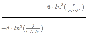
$\Rightarrow K_{1}>-8\cdot ln^{3}(\frac {\delta}{6\cdot N\cdot k^{2}})$
, and we can choose $K_{1}>-6\cdot ln^{3}(\frac {\delta}{6\cdot N\cdot k^{2}})$ to narrow down the interval of probabilistic estimation failure.

➇expand from $K_{1}^{-\frac {1}{3}}<\frac {\varepsilon}{2\cdot N\cdot T\cdot R_{max}}$
$\Rightarrow K_{1}>(\frac {2\cdot N\cdot T\cdot R_{max}}{\varepsilon})^{3}$
, and $K_{1}>(\frac {4\cdot N\cdot T\cdot R_{max}}{\varepsilon})^{3}$ holds for it.

Finally, $K_{1}$=$max((\frac {4\cdot N\cdot T\cdot R_{max}}{\varepsilon})^{3},-6\cdot ln^{3}(\frac {\delta}{6\cdot N\cdot k^{2}}))+1$, after this $K_{1}$ trials over the same state, we are confident to to turn a state from unknown to known or to update its statistics information, we believe that the estimated transitive probability is accurate.

The RMAX Theorem Proof::2

The implicit explore or exploit lemma yields a transitive probability of $\frac {\alpha}{R_{max}}$, we next show that after pure exploration over $K_{2}$ trials on this same state $G_{i}$, we can obtain $K_{1}$ required visits on $G_{i}$.

➀let $X_i$ be the random variable of indicator for each trial, whose value is $1$ iff it transits from $G_{i}$ to $G_{i^{'}}$; or $0$ iff it justs exploits in the same $G_{i}$.

➁let $Z_{i}$=$X_{i}-\frac {\alpha}{R_{max}}$ and $Z_{i}^{'}$=$\frac {\alpha}{R_{max}-X_{i}}$, then $E\lbrack Z_{i}\rbrack$=$0$ and $E\lbrack Z_{i}^{'}\rbrack$=$0$ respectively.

• By Chernoff Bounds For Bernoulli Random Variable
  $P(\vert\sum_{i=1}^{K_{2}}(X_{i}-\frac {\alpha}{R_{max}})\vert>K_{2}^{\frac {1}{3}})<2\cdot e^{-\frac {K_{2}^{-\frac {1}{3}}}{2}}$
  $\Rightarrow P(\vert\sum_{i=1}^{K_{2}}X_{i}-\frac {K_{2}\cdot\alpha}{R_{max}}\vert>K_{2}^{\frac {1}{3}})<2\cdot e^{-\frac {K_{2}^{-\frac {1}{3}}}{2}}$
• To limit the error terms
  Take $2\cdot e^{-\frac {K_{2}^{-\frac {1}{3}}}{2}}<\frac {\delta}{3\cdot N\cdot k^{2}}$
  , and take $\frac {K_{2}\cdot\alpha}{R_max}+K_{2}^{\frac {1}{3}}>K_{1}\cdot N\cdot k^{2}$
  , for totally we have $N\cdot k^{2}\cdot K_{1}$ number of visits to unknown slots. These guarantee that the fail probability less than $\frac {\delta}{3}$, which is much smaller than $\delta$.
• Why $K_{2}^{\frac {1}{3}}$ as the error term instead of $K_{2}^{\frac {2}{3}}$?

  The design of this proof is to find the least $K_{2}$ pure exploration trials, thus guarantees that we could have $K_{1}$ visits on this same state. Since $K_{1}$ contains exploration and exploitation, $K_{2}\leq K_{1}$, therefore, the error term is expressed in terms of $K_{2}^{\frac {1}{3}}$, rather than $K_{2}^{\frac {2}{3}}$!! We want a smaller $K_{2}<K_{1}$ and $K_{2}^{\frac {1}{3}}<K_{1}^{\frac {2}{3}}$.

The RMAX Theorem Proof::3

This section discuss the scenario that we perform $T$-step iterations without learning, that is to say it exploits over $T$ steps, and the optimal expected reward would be $Opt(\prod_{M}(T,\varepsilon))-\varepsilon$.

• The actual return may be lower

  Since the actual reward after execution of the RMAX algorithm would be some distance from optimal reward, it is at most $Opt(\prod_{M}(T,\varepsilon))-\varepsilon$, it is lower than $Opt(\prod_{M}(T,\varepsilon))-\varepsilon$, which is plausible. If we prevent it from exploring, we are at least staying in some local suboptimal.

• We want it to be more closer
  To align the design in above section, we choose the real return of exploitation after $T$-step iterations to be $Opt(\prod_{M}(T,\varepsilon))-\frac {3}{2}\varepsilon$, then it is $\frac {1}{2}\varepsilon$ close to the optimal reward $Opt(\prod_{M}(T,\varepsilon))-\varepsilon$. The RMAX paper upper bound the failure probability by $\frac {\delta}{3}$.

➀take $X_{i}$ to be the actual reward obtained in each trial
➁treat $\mu$ as the optimal reward
➂then by $y_{i}$=$\frac {\mu-X_{i}}{R_{max}}$ could we stablize the standard deviation, since it is bounded by $R_{max}$
➃suppose $Z$=$M\cdot N\cdot T$, where $M>0$, after $Z$ exploitations, the failure probability that the total loss greater than $Z^{\frac {2}{3}}$ is upper bounded by $e^{-\frac {Z^{\frac {1}{3}}}{2}}$

• By Chernoff Bounds For Bernoulli Random Variable
  $P(\sum_{i=1}^{Z}Y_{i}>Z^{\frac {2}{3}})<e^{-\frac {Z^{\frac {1}{3}}}{2}}$
  $\Rightarrow P(\sum_{i=1}^{Z}\frac {\mu-X_{i}}{R_{max}}>Z^{\frac {2}{3}})<e^{-\frac {Z^{\frac {1}{3}}}{2}}$
  $\Rightarrow P(\sum_{i=1}^{Z}\frac {\mu-X_{i}}{Z\cdot R_{max}}>Z^{-\frac {1}{3}})<e^{-\frac {Z^{\frac {1}{3}}}{2}}$
  $\Rightarrow P(\sum_{i=1}^{Z}\frac {\mu-X_{i}}{Z}>\frac {R_{max}}{Z^{\frac {1}{3}}})<e^{-\frac {Z^{\frac {1}{3}}}{2}}$

➄by choosing $M$ such that
$\frac {R_{max}}{Z^{\frac {1}{3}}}<\frac {\varepsilon}{2}$ and $e^{-\frac {Z^{\frac {1}{3}}}{2}}<\frac {\delta}{3}$
$\Rightarrow Z>(\frac {2\cdot R_Max}{\varepsilon})^{3}$ and $Z>6\cdot ln^{3}(\frac {\delta}{3})$,
We thus have the failure probability less than $\frac {\delta}{3}$ for the real return obtained is $\frac {\varepsilon}{2}$ far away from the optimal reward.

Addendum

➀R-max: A General Polynomial Time Algorithm for Near-Optimal Reinforcement Learning, Ronen I. Brafman, CS in Ben-Gurion University, Moshe Tennenholtz, CS in Stanford University

Model-Based RL Algorithm RMAX - Part 3

28 Feb 2020

Prologue To Model-Based RL Algorithm RMAX - Part 3

The major insight behind the RMAX algorithm is the property that it is always either optimal or it leads to efficient learning.

The RMAX Property: Implicit Explore Or Exploit

At each point during the learning process, the agent can either choose one of below:
➀to exoplore to other states, or
➁to exploit over the same state.

If the agent follows an optimal policy with respect to the model it maintains for $T$ steps, it will either attain near-optimal average reward or it will update the statistics for one of the unknown states with sufficient high probability.

The choice in between exploration and exploitation is implicit.

Prerequisites For Implicit Explore Or Exploit

[1] Basic definition

Before we prove the choice in between exploration and exploitation is implicit, there shall exist definition of prerequisites to make this theorem of property more concrete:
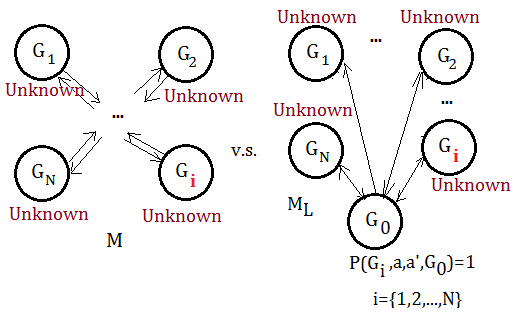
➀define $M$ to be a stochastic game.
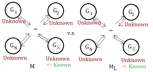
➁define $L$ to be a set of unknown states in the form of $(G_{i},a,a^{'})$, that is to say $G_{i}$ is an unknown state.
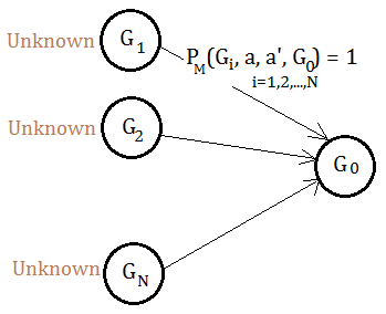
➂define $M_{L}$ to be a stochastic game identical to $M$, except that $M_{L}$ contains an extra $G_{0}$ state with $P(G_{i},a,a^{'},G_{0})$=$1$ for any $G_{i}\in L$, and the reward is $R_{max}$ for the agent, and $0$ for the adversary.

[2] More detail

Take a more close look in above definition:

• $M_{L}$ is the deduced model of $M$

  ➀in the beginning of RMAX algorithm, we treat all states as unknown.

• After explore or exploit over some horizon in the given sampling of data:
  ➀the reward of known states in $M_{L}$ is at least as large as in $M$, in the instance of $G_{K}$.
  ➁the optimal policy deduced out in $M_{L}$ is also optimal with respect to $M$, could be applied onto $M$. Because $M_{L}$ is almost the same as $M$, except that $M_{L}$ has an extra $G_{0}$ with transitive probability to $1$ from all other states to $G_{0}$.

Base on all above, we’d like to prove the nature of implicit or explicit explore will either attains optimal reward or leads to efficient learning.

Implicit Explore Or Exploit Lemma

Construct the scenario by below list conditions:
➀let $M$ and $M_{L}$ be the same models described above
➁let $\rho$ be any arbitrary policy of the adversary
➂let $0<\alpha<1$
➃let $s$ be any state

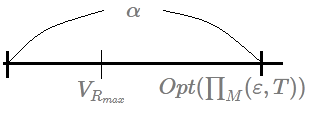
When you deduce out an optimal policy $R_{-max}^{ML}$ on the simulated model $M_{L}$ and apply it on the target model $M$, you will either have one of below holds:
➀$V_{R_{max}}>Opt(\prod_{M}(\varepsilon,T))-\alpha$, where $V_{R_{max}}$ is just the expected $T$-step average reward for $R_{-max}^{ML}$ applied on $M$
➁an unknown entry will be played in the course of running $R_{-max}^{ML}$ on $M$ for $T$ steps with the probability of at least $\frac {\alpha}{R_{max}}$

Such deduced out policy $R_{-max}^{ML}$ on $M_{L}$ is the RMAX policy!!

proof::mjtsai1974

Below illustrates the majority of the lemma:

[1]Begin from the difference in between $V_{R_{max}}$ and $Opt(\prod_{M}(\varepsilon,T))$

➀by artificial design we’d like to have our expected average reward after the execution of RMAX to be greater than the optimal reward of the optimal policy minus $\alpha$, because that would be a little more close to the optimal policy’s reward.

➁$\vert U_{M}(\varepsilon,R_{-max}^{M_{L}},s,T)-U_{M}(\varepsilon,\pi,s,T)\vert$
=$\vert\sum_{q}P(q)\cdot V_{M}(R_{-max}^{M_{L}},q)+\sum_{r}P(r)\cdot V_{M}(R_{-max}^{M_{L}},r)$
$-\sum_{q}P(q)\cdot V_{M}(\pi,q)-\sum_{r}P(r)\cdot V_{M}(\pi,r)\vert$
$\leq\vert\sum_{q}P(q)\cdot V_{M}(R_{-max}^{M_{L}},q)-\sum_{q}P(q)\cdot V_{M}(\pi,q)\vert$
$\;\;$+$\vert\sum_{r}P(r)\cdot V_{M}(R_{-max}^{M_{L}},r)-\sum_{r}P(r)\cdot V_{M}(\pi,r)\vert$

where we have $p$=$\{q,r\}$, $q$ is the path containing all known states, whereas $r$ is the path leads to unknown target/next state.

and $\vert a+b-c-d\vert\leq\vert a-c\vert+\vert b-d\vert$, since $a-c$ might be negative!!

➂due to $q$ is the path to all known states, we have it holds $\vert\sum_{q}P(q)\cdot V_{M}(R_{-max}^{M_{L}},q)-\sum_{q}P(q)\cdot V_{M}(\pi,q)\vert$=$0$

➃the inequality becomes
$\vert U_{M}(\varepsilon,R_{-max}^{ML},s,T)-U_{M}(\varepsilon,\pi,s,T)\vert$
$\leq\vert\sum_{r}P(r)\cdot V_{M}(R_{-max}^{M_{L}},r)-\sum_{r}P(r)\cdot V_{M}(\pi,r)\vert$
$\leq\alpha$
$\leq\sum_{r}P(r)\cdot R_{max}$

and $\alpha\neq 0$, for some $\alpha$ under the condition that $M_{L}\rightarrow_{\alpha}M$, this just holds for $R_{max}$ is just the upper bound for unknown state in RMAX algorithm.

➄then, we have $P(r)\geq\frac {\alpha}{R_{max}}$ just holds

We next to go back to prove the artificial target that the real reward of RMAX is within optimal reward minus something, say $\alpha$.

[2]The real reward of RMAX is within optimal reward minus $\alpha$

➀from above deduction, we already have
$\vert U_{M}(\varepsilon,R_{-max}^{M_{L}},s,T)-U_{M}(\varepsilon,\pi,s,T)\vert\leq\alpha$

➁take off the absolute function, we have below inequality
$U_{M}(\varepsilon,\pi,s,T)-\alpha\leq U_{M}(\varepsilon,R_{-max}^{ML},s,T)\leq U_{M}(\varepsilon,\pi,s,T)+\alpha$

For the left part, it just proves, and we need to step over to the right side.

[3]Step over to the right side

➀since $U_{M_{L}}(\varepsilon,R_{-max}^{M_{L}},s,T)$ is at least as large as $U_{M}(\varepsilon,\pi,s,T)$, see above prerequisites section for detail, therefore it holds
$U_{M}(\varepsilon,\pi,s,T)\leq U_{M_{L}}(\varepsilon,R_{-max}^{M_{L}},s,T)$

➁we have it that
$U_{M}(\varepsilon,R_{-max}^{M_{L}},s,T)\leq U_{M}(\varepsilon,\pi,s,T)+\alpha\leq U_{M_{L}}(\varepsilon,R_{-max}^{M_{L}},s,T)+\alpha$

➂for $R_{-max}^{ML}$ deduced on $M_{L}$, its reward would be at least as large as the optimal policy in $M$, therefore,
$U_{M}(\varepsilon,R_{-max}^{M_{L}},s,T)-\alpha\leq U_{M_{L}}(\varepsilon,R_{-max}^{M_{L}},s,T)$

➃well, we have the deduced out $R_{-max}^{M_{L}}$ on $M_{L}$ is also the optimal policy with respect to $M$, then
$U_{M}(\varepsilon,\pi,s,T)-\alpha\leq U_{M_{L}}(\varepsilon,R_{-max}^{M_{L}},s,T)$

➄as a result that the reward obtained after the execution of $R_{-max}^{M_{L}}$ on $M$ is no less than the reward btained by $R_{-max}^{M_{L}}$ on $M_{L}$, hence
$U_{M}(\varepsilon,\pi,s,T)-\alpha\leq U_{M_{L}}(\varepsilon,R_{-max}^{M_{L}},s,T)\leq U_{M}(\varepsilon,R_{-max}^{M_{L}},s,T)$

We finally go back to the left side of $U_{M}(\varepsilon,\pi,s,T)-\alpha\leq U_{M}(\varepsilon,R_{-max}^{M_{L}},s,T)$ from the righ side.

Addendum

➀R-max: A General Polynomial Time Algorithm for Near-Optimal Reinforcement Learning, Ronen I. Brafman, CS in Ben-Gurion University, Moshe Tennenholtz, CS in Stanford University

Model-Based RL Algorithm RMAX - Part 2

23 Feb 2020

Prologue To Model-Based RL Algorithm RMAX - Part 2

The RMAX theorem guarantees that the execution of algorithm will attain $-2\cdot\varepsilon$ close to optimal expected return in polynomial time, whereas the algorithm is developed by constructing a simulated model plugging with an extra fictitious $G_{0}$ state to approximate the target model. To validate the algorithm, this article would like to prove that the difference of the expected returns in between the simulated and the target model is infinitesimal.

$\alpha$ Approximation

Given that $M$ and $M^{'}$ are 2 distinct stochastic games over the same set of states and actions, then $M^{'}$ is $\alpha$ approximation of $M$ if below holds for every state $s$:
➀$P_{M}(s,a,a^{'},s^{'})-\alpha\leq P_{M^{'}}(s,a,a^{'},s^{'})\leq P_{M}(s,a,a^{'},s^{'})+\alpha$
, where $P_{M}(s,a,a^{'},s^{'})$ is the probabilistic transition for the agent from state $s$ to $s^{'}$ by choosing action $a$, and the adversary chooses action $a^{'}$ in model $M$, the same for $P_{M^{'}}(s,s^{'},a,a^{'})$ is the same.
➁for every state $s$, the same stage game is associated with $s$ in $M$ and $M^{'}$, the rewards would be identical.

Approximation Makes Small Difference

Let $M$ and $M^{'}$ be stochastic games over $N$ states, where $M^{'}$ is an $\frac {\varepsilon}{N\cdot T\cdot R_{max}}$ approximation of $M$, then for every state $s$, agent policy $\pi$, adversary policy $\rho$, we have that

• $\left|U_{M^{'}}(s,\pi,\rho,T)-U_{M}(s,\pi,\rho,T)\right|\leq\varepsilon$
  , where $U_{M}(s,\pi,\rho,T)$ is the optimal expected reward with regards to agent policy $\pi$, adversary policy $\rho$, given that they are from state $s$, make state transitions over $T$ steps.

proof::mjtsai1974

➀begin from
$\left|U_{M^{'}}(s,\pi,\rho,T)-U_{M}(s,\pi,\rho,T)\right|$
=$\sum_{p}\left|P_{M^{'}}(p)\cdot U_{M^{'}}(p) - P_{M}(p)\cdot U_{M}(p)\right|$

, where $p$ is the path starting from each state $s$, totally $N$ states, after ranging from $s$, make state transition of $T$ steps.

➁each such optimal expexted reward of path $p$ in $M^{'}$ could be expressed as:
$\sum_{s}\sum_{s’}P_{M^{'}}(s,a,a^{'},s^{'})\cdot U_{M^{'}}(s^{'})$

, where $U_{M^{'}}(s^{'})$=$\sum_{i=1}^{T}\gamma^{i-1}\cdot V_{M^{'}}(S_{i}^{'})$

➂origin formula in ➀ becomes:
$\sum_{s}\sum_{s’}(P_{M^{'}}(s,a,a^{'},s^{'})\cdot U_{M^{'}}(s^{'})$-$P_{M}(s,a,a^{'},s^{'})\cdot U_{M}(s^{'}))$

, where $s$=$\{s_{1},s_{2},…,s_{N}\}$

➃we are given $M^{'}$ is an $\alpha$ approximation of $M$, and
$U_{M^{'}}(s^{'})$=$\sum_{i=1}^{T}\gamma^{i-1}\cdot V_{M^{'}}(s_{i}^{'})\leq\sum_{i=1}^{T}V_{M^{'}}(s^{'})$ must hold

➄$\left|U_{M^{'}}(s,\pi,\rho,T)-U_{M}(s,\pi,\rho,T)\right|$
=$\sum_{s}\sum_{s’}(P_{M^{'}}(s,a,a^{'},s^{'})\cdot U_{M^{'}}(s^{'})$-$P_{M}(s,a,a^{'},s^{'})\cdot U_{M}(s^{'}))$
=$\sum_{s}\sum_{s’}(P_{M^{'}}(s,a,a^{'},s^{'})\cdot\sum_{i=1}^{T}V_{M^{'}}(s^{'})$-$P_{M}(s,a,a^{'},s^{'})\cdot\sum_{i=1}^{T}V_{M}(s^{'}))$
=$\sum_{s}\sum_{s’}(P_{M^{'}}(s,a,a^{'},s^{'})$-$P_{M}(s,a,a^{'},s^{'})\cdot T\cdot(V_{M^{'}}(s^{'})-V_{M}(s^{'})))$
$\leq\sum_{s}\sum_{s’}(\frac {\varepsilon}{N\cdot T\cdot R_{max}}\cdot T\cdot(V_{M^{'}}(s^{'})-V_{M}(s^{'})))$
$\;\;$…by given $M^{'}$ is an $\frac {\varepsilon}{N\cdot T\cdot R_{max}}$ approximation of $M$
$\leq\sum_{s}\sum_{s’}(\frac {\varepsilon}{N\cdot T\cdot R_{max}}\cdot T\cdot R_{max})$
$\;\;$…all optimal expected rewards are bounded by $R_{max}$ in this algorithm, so is the difference
$\leq N\cdot\frac {\varepsilon}{N\cdot T\cdot R_{max}}\cdot T\cdot R_{max}$=$\varepsilon$
$\;\;$…totally $N$ such states, each distinct $s$ has lots of $s^{'}$ as its next state, the transitive probability of the same $s$ could then be summed up to $1$, thus $\sum_{s}\sum_{s^{'}}$=$N$

Addendum

➀R-max: A General Polynomial Time Algorithm for Near-Optimal Reinforcement Learning, Ronen I. Brafman, CS in Ben-Gurion University, Moshe Tennenholtz, CS in Stanford University

Model-Based RL Algorithm RMAX - Part 1

08 Feb 2020

Prologue To Model-Based RL Algorithm RMAX - Part 1

RMAX is a simple model-based reinforcement learning algorithm that can attain near-optimal average reward in polynomial time.

MDP Model Construct From Given Data

[Question]

Here is the condition, suppose you are given:
➀a sample of probabilistic transitions and immediate rewards pertaining to a MDP model
➁the full set of states is known in advance
➂but, only the contour, exclusive of the path in between states
➃all states are initialized as unknown

We don’t have the whole MDP yet, what would you do to construct a complete MDP model? What do we do along the way?

[Answer]

We would be able to refer to the Temporal Difference Learning - Part 1, Temporal Difference Learning - Part 2, Temporal Difference In Q Form in my prior post, which is a model-free algorithm.

However, we are given the full set of states, the suggestion would be made to use the RMAX, which is a model-based algorithm.

Before We Enter RMAX Algorithm

[1] Brief description

The approach used by RMAX has been refered to as the optimism in the face of uncertainty heuristic. It propose a specific approach in which the choice in between exploration and exploitation is implicit.

The major insight behind this algorithm is the optimal policy with respect to the agent’s fictitious model has a very interesting and useful property that it is always optimal or it leads to efficient learning.

[2] Preliminaries

The RMAX algorithm was presented in the context of a model called stochastic game in R-max: A General Polynomial Time Algorithm for Near-Optimal Reinforcement Learning, Ronen I. Brafman, CS in Ben-Gurion University, Moshe Tennenholtz, CS in Stanford University. Stochastic game is more general than MDP, because it doesn't necessarily assume that the environment is stochastic.

Please recall in MDP, the execution of the action might not go as well as it has been expected, it is a stochastic environment.

A stochastic game is a model of multi-agent interaction. It has a set of players, each of whom chooses some action to perform from within a given set of actions. As a result of the combinatory choices, some outcome is obtained and is described numerically in the form of a payoff vector, vector of values, one for each of the players.

The RMAX was developed on 2 palyers, fixed-sum games, in which the sum of values in the payoff vector is constant. The player under our control is called the agent, whereas the other one is the adversary.

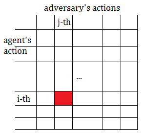
The game is commonly described in strategic form of matrix, the rows of a matrix correspond to the agent’t actions and the columns correspond to the adversary’s actions. The entry of row i and column j contains the rewards obtained for the agent chooses i-th and the adversary chooses the j-th action.

In stochastic game, the player plays a sequence of standard games, which represents the states in normal MDP. After playing a game, it obtains rewards and transits to a new game(or maybe stay in the same place), in both models, actions lead to transitions between states, such similarity could be found.

You could treat MDP as an stochastic game in which the adversary has only a single action at each state.

The RMAX Algorithm

[Input]

Below are the basic defines:
➀$N$: the number of stage games(or states).
➁$k$: the number of actions for each state.
➂$\varepsilon$: the error bound.
➃$\delta$: the algorithm’s failure probability.
➄$R_{max}$: the upper bound on the reward function.
➅$T$: the maximum number of steps for the optimal policy of the algorithm to get $\varepsilon$ close to the average expected(undiscounted) reward.

[Inintialize]

Initialize by constructing a model $M^{'}$ consisting of
➀$N+1$ stage games, ${G_{0},G_{1},…,G_{N+1}}$, corresponding to the real states.
➁$k$ actions, ${a_{1},…,a_{k}}$, which would then be played by the agent and the adversary.
➂set each $G_{i}$ in unknown status.

Where the $G_{0}$ is an additional fictitious game, of which we are in need to initialize the probability for each $G_{i}$ to transite to $G_{0}$ by the agent choosing action $a$ and the adversary choosing $a^{'}$ to be $1$, that is $P_{M}(G_{i},G_{0},a,a^{'})$=$1$, $i$=${0,1,…,N}$.

Cautions must be made that the RMAX Algorithm is using the constructed model $M^{'}$ to approximate the real model $M$, that’s why it is $P_{M}(G_{i},G_{0},a,a^{'})$, not $P_{M^{'}}(G_{i},G_{0},a,a^{'})$.

[Repeat]

• Compute an optimal $T$-step policy and take action:
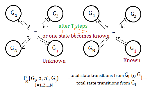
  ➀execute this policy for $T$-steps.
  ➁or until a new entry of $G_{i}$ becomes known.

• Keep track of action execution results:
  ➀update the reward thus obtained upon state transition from $G_{i}$ to $G_{j}$ after the execution of joint action of actions $a$ and $a^{'}$ for its very first time.
  ➁update the set of states thus reached in accordance to each action pair $(a,a^{'})$ in $G_{i}$.
  ➂if this entry of $G_{i}$ has been explored over $K_{1}$ times, in other words, the set of states reached from this $G_{i}$ contains $K_{1}$ elements, mark this $G_{i}$ as known, and update the transition probabilities in the unit of distinct transition from $G_{i}$ to $G_{j}$.

Where $K_{1}$=$max((\frac {4\cdot N\cdot T\cdot R_{max}}{\varepsilon})^{3},-6\cdot ln^{3}(\frac {\delta}{6\cdot N\cdot k^{2}}))+1$, which would then be proved in the following secction.

[Brief summary]

The RMAX algorithm constructs a model $M^{'}$ to approximate the real model $M$, by initializing all states as unknown and the probability for each $G_{i}$ of all action pairs $(a,a^{'})$ to $G_{0}$ be $1$.

Based on model $M^{'}$, compute an optimal $T$-step policy, follow from the departuring state in each eposide, say $G_{i}$, keep record of all states reached in accordance to the execution of action pairs $(a, a^{'})$.

At the moment $T$ steps has been reached or the departuring $G_{i}$ turns into known, update the probabilistic transition from this state to its next states. Each time, after such $G_{i}$ has been updated, recompute an optimal $T$-step policy and repeat.

Addendum

➀Exploring Deterministics MDP, Charles IsBell, Michael Littman, Reinforcement Learning By Georgia Tech(CS8803)
➁R-max: A General Polynomial Time Algorithm for Near-Optimal Reinforcement Learning, Ronen I. Brafman, CS in Ben-Gurion University, Moshe Tennenholtz, CS in Stanford University

Chernoff Bounds For Arbitrary Random Variable

23 Dec 2019

Prologue To The Chernoff Bounds For Arbitrary Random Variable

There are many Chernoff bounds as a result. This article develops the tail bound on the independent arbitrary random variable with outcome ranging from 0 to 1, that is $\lbrack 0,1\rbrack$.

The Error Probability After Test

[The given condition]

Suppose we are given
➀$X_{1}$,$X_{2}$,…,$X_{n}$ to be independent random variables with values in $\lbrack 0,1\rbrack$.
➁$X$=$X_{1}$+$X_{2}$+…+$X_{n}$
➂$E\lbrack X \rbrack$=$\mu$

These $X_{1}$,…,$X_{n}$ needs not to be Bernoulli ranodm variables, but they must be independent.

[Question]

Then, for every $\varepsilon$>$0$, what is the upper and lower bound for
➀$P(X\geq (1+\delta)\cdot\mu)$=$P(X\geq \mu+\varepsilon)$
➁$P(X\leq (1-\delta)\cdot\mu)$=$P(X\leq \mu-\varepsilon)$
, where $\varepsilon$=$\delta\cdot\mu$

The Upper Bound On Error Probability

Still, it is asking the upper bound on error probability, when target value $X$ is greater than the expect value $\mu$, and we’d like to bound it on the upper side.

The major difference is that these random variables fall within $\lbrack 0,1\rbrack$, not the Bernoulli values $0$ or $1$. Here is the idea:
➀take $Y_{i}$=$X_{i}$-$E\lbrack X_{i} \rbrack$
➁take $X$=$\sum_{1}^{n}X_{i}$,$E\lbrack X \rbrack$=$\mu$=$\sum_{1}^{n}E\lbrack X_{i} \rbrack$
➂take $Y$=$\sum_{1}^{n}Y_{i}$
➃$P(X\geq\mu+\varepsilon)$
=$P(X-\mu\geq\varepsilon)$
=$P(\sum_{1}^{n}(X_{i}-E\lbrack X_{i} \rbrack)\geq\varepsilon)$
=$P(Y\geq\varepsilon)$
=$P(e^{t\cdot Y}\geq e^{t\cdot\varepsilon})$…for any $t>0$
$\leq\frac {E\lbrack e^{t\cdot Y}\rbrack}{e^{t\cdot\varepsilon}}$, and $E\lbrack Y_{i}\rbrack$=$0$

Further expand
$E\lbrack e^{t\cdot Y}\rbrack$
=$E\lbrack e^{\sum_{1}^{n} t\cdot Y_{i}}\rbrack$
=$E\lbrack \prod_{1}^{n} e^{t\cdot Y_{i}}\rbrack$
=$\prod_{1}^{n}E\lbrack e^{t\cdot Y_{i}}\rbrack$

Thus, $P(X\geq \mu+\varepsilon)\leq\frac {\prod_{1}^{n}E\lbrack e^{t\cdot Y_{i}}\rbrack}{e^{t\cdot\varepsilon}}$ is left to bound the term $E\lbrack e^{t\cdot Y_{i}}\rbrack$.
➀$D_{y}e^{t\cdot Y_{i}}$=$t\cdot e^{t\cdot Y_{i}}>0$
➁$D_{y}t\cdot e^{t\cdot Y_{i}}$=$t^{2}\cdot e^{t\cdot Y_{i}}>0$
$e^{t\cdot Y_{i}}$ is a convex function, it concaves up, by the 2nd derivative greater than 0.

Suppose there exists a line $a+b\cdot y$ passing through the curve of $e^{t\cdot Y_{i}}$ at the points $(1,e^{t})$ and $(-1,e^{-t})$, that is
$a$+$b$=$e^{t}$
$a$-$b$=$e^{-t}$
$\Rightarrow$solve above equation, could we obtain $a$=$\frac {e^{t}+e^{-t}}{2}$, $b$=$\frac {e^{t}-e^{-t}}{2}$

We can claim that within $\lbrack -1,1\rbrack$
$e^{t\cdot Y_{i}}\leq a+b\cdot Y_{i}$
$\Rightarrow E\lbrack e^{t\cdot Y_{i}}\rbrack\leq E\lbrack a+b\cdot Y_{i}\rbrack$
$\Rightarrow E\lbrack e^{t\cdot Y_{i}}\rbrack\leq a + b\cdot E\lbrack Y_{i}\rbrack$
$\Rightarrow E\lbrack e^{t\cdot Y_{i}}\rbrack\leq a + b\cdot 0$, where $E\lbrack Y_{i}\rbrack$=$0$
$\Rightarrow E\lbrack e^{t\cdot Y_{i}}\rbrack\leq a$
$\Rightarrow E\lbrack e^{t\cdot Y_{i}}\rbrack\leq \frac {e^{t}+e^{-t}}{2}$

By using Taylor expansion of $e^{t}$, we can simplify the bounding:
$e^{x}$=$1$+$\frac {x^{1}}{1!}$+$\frac {x^{2}}{2!}$+$\frac {x^{3}}{3!}$+…, then
$\frac {e^{t}+e^{-t}}{2}$
=$\frac {1}{2}\cdot\lbrack$+$1$+$\frac {t^{1}}{1!}$+$\frac {t^{2}}{2!}$+$\frac {t^{3}}{3!}$+$\frac {t^{4}}{4!}$+… +$1$+$\frac {(-t)^{1}}{1!}$+$\frac {(-t)^{2}}{2!}$+$\frac {(-t)^{3}}{3!}$+$\frac {(-t)^{4}}{4!}$+…+$\rbrack$
=$1$+$\frac {t^{2}}{2!}$+$\frac {t^{4}}{4!}$+$\frac {t^{6}}{6!}$+…
$\leq 1$+$\frac {t^{2}}{2\cdot 1!}$+$\frac {t^{4}}{2^{2}\cdot 2!}$+$\frac {t^{6}}{2^{3}\cdot 3!}$+…
$\leq 1$+$\frac {\frac {t^{2}}{2}}{1!}$+$\frac {(\frac {t^{2}}{2})^{2}}{2!}$+$\frac {(\frac {t^{2}}{2})^{3}}{3!}$+…
$\leq e^{\frac {t^{2}}{2}}$

Therefore, $e^{t\cdot Y_{i}}\leq e^{\frac {t^{2}}{2}}$,
$\prod_{1}^{n}E\lbrack e^{t\cdot Y_{i}}\rbrack$
=$E\lbrack e^{t\cdot (Y_{1}+Y_{2}+…+Y_{n})}\rbrack$
=$E\lbrack e^{n\cdot t\cdot Y_{i}}\rbrack$
$\leq E\lbrack e^{\frac {t^{2}}{2}}\rbrack$

Back to the inequality:
$P(X\geq \mu+\varepsilon)$
$\leq\frac {\prod_{1}^{n}E\lbrack e^{t\cdot Y_{i}}\rbrack}{e^{t\cdot\varepsilon}}$
$\leq\frac {E\lbrack e^{\frac {t^{2}}{2}}\rbrack}{e^{t\cdot\varepsilon}}$
$\leq e^{\frac {t^{2}}{2}-t\cdot\varepsilon}$

Next would be:
➀ask for the maximum value of $\frac {t^{2}}{2}-t\cdot\varepsilon$, take its 1st order differentiation, set it to 0, figure out such $t$:
$D_{t}(\frac {t^{2}}{2}-t\cdot\varepsilon)$=$0$
$\Rightarrow n\cdot t-\varepsilon$=$0$
$\Rightarrow t$=$\frac {\varepsilon}{n}$

➁take $t$=$\frac {\varepsilon}{n}$ in $e^{\frac {t^{2}}{2}-t\cdot\varepsilon}$, then
$e^{\frac {n\cdot \frac {\varepsilon^{2}}{n^{2}}}{2}-\frac {\varepsilon}{n}\cdot\varepsilon}$
=$e^{\frac {\varepsilon^{2}}{2n}-\frac {\varepsilon^{2}}{n}}$
=$e^{-\frac {\varepsilon^{2}}{2n}}$

Finally, we prove $P(X\geq \mu+\varepsilon)\leq e^{-\frac {\varepsilon^{2}}{2n}}$ in this upper bound for error probability.

The Lower Bound On Error Probability

It is asking the error probability when target value $X$ is less than the expect value $\mu$, and we’d like to bound it on the lower side.
$P(X\leq \mu-\varepsilon)$
=$P(X-\mu\leq -\varepsilon)$
=$P(-X+\mu\geq \varepsilon)$
=$P(-X\geq -\mu+\varepsilon)$

It is much similar to the upper bound expression, here is the idea again:
➀take $Y_{i}^{'}$=$E\lbrack X_{i} \rbrack$-$X_{i}$
➁take $X$=$\sum_{1}^{n}X_{i}$,$E\lbrack X \rbrack$=$\mu$=$\sum_{1}^{n}E\lbrack X_{i} \rbrack$
➂take $Y^{'}$=$\sum_{1}^{n}Y_{i}^{'}$
➃$P(X\leq \mu-\varepsilon)$
=$P(-X\geq -\mu+\varepsilon)$
=$P(Y^{'}\geq \varepsilon)$
=$P(e^{t\cdot Y^{'}}\geq e^{t\cdot\varepsilon})$…for any $t>0$
$\leq\frac {E\lbrack e^{t\cdot Y^{'}}\rbrack}{e^{t\cdot\varepsilon}}$

With similar deduction in upper bound would we obtain the same expression for lower bound:
$P(X\leq \mu-\varepsilon)\leq e^{-\frac {\varepsilon^{2}}{2n}}$

By symmetrical distribution, $P(X-\mu\leq -\varepsilon)$ is the opposite direction to $P(X-\mu\geq \varepsilon)$, its lower bound of error probability would be no more than $e^{\frac {t^{2}}{2}-t\cdot\varepsilon}$
$P(X\leq \mu-\varepsilon)$
=$P(X-\mu\leq -\varepsilon)$

Illustration: Chernoff bound For Bernoulli versus arbitrary Random Variables::mjtsai1974

[The major point] Why the proof in Chernoff bound for Bernoulli is inadequate in arbitrary random variables? Can we use the proof in Chernoff bound for Bernoulli in arbitrary random variable?

If not, why?

The Bernoulli random variable has only two values, $0$ and $1$, while arbitrary random variable has values falling withing $\lbrack 0,1\rbrack$. It seems that probabilistic error tolerance in arbitrary random variables requires much more precision concern in approximation, which would be shown in my next proof.

[1] The fault tolerance $\delta$ of upper and lower bound

From the proof in Chernoff Bounds For Bernoulli Random Variable, we see that
➀$P(X>(1+\delta)\cdot\mu)$<$e^{((e^{t}-1)-t\cdot (1+\delta))\cdot\mu}$
➁$P(X<(1-\delta)\cdot\mu)$<$e^{(-1-t\cdot\delta)\cdot\mu}$

Next would be to inspect the fault tolerance $\delta$ in Chernoff bounds for Bernoulli random variable for any given $t$>$0$, based on the convex property used in the proof of Chernoff bounds for arbitrary random variable.

[1.1] The fault tolerance $\delta$ of upper bound

➀$D_{t}e^{((e^{t}-1)-t\cdot (1+\delta))\cdot\mu}$
=$(e^{t}-(1+\delta))\cdot\mu\cdot e^{((e^{t}-1)-t\cdot (1+\delta))\cdot\mu}$
➁$D_{t}^{2}e^{((e^{t}-1)-t\cdot (1+\delta))\cdot\mu}$
=$(e^{t}\cdot\mu+(e^{t}-(1+\delta))^{2})\cdot e^{((e^{t}-1)-t\cdot (1+\delta))\cdot\mu}$

Since $D_{t}^{2}e^{((e^{t}-1)-t\cdot (1+\delta))\cdot\mu}\geq 0$ alswys holds, this upper bound of $e^{((e^{t}-1)-t\cdot (1+\delta))\cdot\mu}$ in Chernoff bounds for Bernoulli random variable is a convex function, which concaves up.

➂suppose $c$+$d\cdot t$ pass through $e^{((e^{t}-1)-t\cdot (1+\delta))\cdot\mu}$ at $(0,1)$ and $(1,e^{e-2-\delta})$…for $t$>$0$
$c$+$d\cdot 0$=$1$…$t$=$0$
$c$+$d$=$e^{e-2-\delta}$…$t$=$1$
$\Rightarrow c=1$ and $d$=$e^{e-2-\delta}$-$1$, thus it is
$1$+$(e^{e-2-\delta}-1)\cdot t$

➃we’d like to figure out fault tolerance of $\delta$ for any $t$>$0$, that is to express $t$ in terms of $\delta$:
$D_{t}(1+(e^{e-2-\delta}-1)\cdot t)$=$0$
$\Rightarrow e^{e-2-\delta}-1$=$0$
$\Rightarrow e^{e-2-\delta}$=$1$
$\Rightarrow e-2-\delta$=$0$
$\Rightarrow \delta$=$e-2$…$e$=$2.71828182…$
$\Rightarrow \delta$=$0.71828182…$

For whatever $0<t\leq 1$ we are using, the fault tolerance expressed by $\delta$ could be probabilistically up to almost $0.718$, might not be an inappropriate choice.

[1.2] The fault tolerance $\delta$ of lower bound

➀$D_{t}e^{(-1-t\cdot\delta)\cdot\mu}$=$-\delta\cdot\mu\cdot e^{(-1-t\cdot\delta)\cdot\mu}$
➁$D_{t}^{2}e^{(-1-t\cdot\delta)\cdot\mu}$=$(-\delta\cdot\mu)^{2}\cdot e^{(-1-t\cdot\delta)\cdot\mu}$

Since $(-\delta\cdot\mu)^{2}\cdot e^{(-1-t\cdot\delta)\cdot\mu}\geq 0$ always holds, this lower bound of $e^{(-1-t\cdot\delta)\cdot\mu}$ in Chernoff bounds for Bernoulli random variable is a convex function, which concaves up.

➂suppose $c$+$d\cdot t$ pass through $e^{(-1-t\cdot\delta)\cdot\mu}$ at $(0,e^{-\mu})$ and $(1,e^{(-1-\delta)\cdot\mu})$, then
$c$+$d\cdot 0$=$e^{-\mu}$…$t$=$0$
$c$+$d$=$e^{(-1-\delta)\cdot\mu}$
$\Rightarrow c$=$e^{-\mu}$ and $d$=$e^{(-1-\delta)\cdot\mu}$-$e^{-\mu}$, thus it is
$e^{-\mu}$+$(e^{(-1-\delta)\cdot\mu}-e^{-\mu})\cdot t$

➃we’d like to figure out fault tolerance of $\delta$ for any $t$>$0$, that is to express $t$ in terms of $\delta$:
$D_{t}(e^{-\mu}+(e^{(-1-\delta)\cdot\mu}-e^{-\mu})\cdot t)$=$0$
$\Rightarrow e^{(-1-\delta)\cdot\mu}-e^{-\mu}$=$0$
$\Rightarrow e^{(-1-\delta)\cdot\mu}$=$e^{-\mu}$
$\Rightarrow (-1-\delta)\cdot\mu$=$-\mu$
$\Rightarrow \delta$=$0$

For whatever $0<t\leq 1$ we are using, the fault tolerance expressed by $\delta$ could only be to $0$, might be an inappropriate choice in error probability evaluation.

[2] The existence of $t$ in upper and lower bound

Succeeding to above section, this article would like to ask for $t$, such that we can have an ideal upper/lower bound, for $\delta$ in $\lbrack -1,1\rbrack$:
➀$P(X>(1+\delta)\cdot\mu)$<$e^{((e^{t}-1)-t\cdot (1+\delta))\cdot\mu}$
➁$P(X<(1-\delta)\cdot\mu)$<$e^{(-1-t\cdot\delta)\cdot\mu}$

[2.1] The validity of $t$ in upper bound

➀$D_{\delta}^{2}e^{((e^{t}-1)-t\cdot (1+\delta))\cdot\mu}\geq 0$
$e^{((e^{t}-1)-t\cdot (1+\delta))\cdot\mu}$ is a convex function.

➁suppose $c$+$d\cdot\delta$ pass through $e^{((e^{t}-1)-t\cdot (1+\delta))\cdot\mu}$ at $(-1,e^{(e^{t}-1)\cdot\mu})$ and $(1,e^{(e^{t}-1-2\cdot t)\cdot\mu})$, then:
$c$=$\frac {e^{(e^{t}-1-2\cdot t)\cdot\mu}+e^{(e^{t}-1)\cdot\mu}}{2}$
$d$=$\frac {e^{(e^{t}-1-2\cdot t)\cdot\mu}-e^{(e^{t}-1)\cdot\mu}}{2}$

➂we’d like to deduct out the expression of $t$ for any $-1\leq\delta\leq 1$, that is to express $\delta$ in terms of $t$:
$D_{\delta}(c+d\cdot\delta)$=$0$
$\Rightarrow d$=$0$
$\Rightarrow \frac {e^{(e^{t}-1-2\cdot t)\cdot\mu}-e^{(e^{t}-1)\cdot\mu}}{2}$=$0$
$\Rightarrow e^{(e^{t}-1-2\cdot t)\cdot\mu}$=$e^{(e^{t}-1)\cdot\mu}$
$\Rightarrow (e^{t}-1-2\cdot t)\cdot\mu$=$(e^{t}-1)\cdot\mu$
$\Rightarrow e^{t}-1-2\cdot t$=$(e^{t}-1)$
$\Rightarrow t$=$0$, which is a contradiction, for $t>0$ is the must be condition in proof.

[2.2] The validity of $t$ in lower bound

➀$D_{\delta}^{2}e^{(-1-t\cdot\delta)\cdot\mu}\geq 0$
$e^{(-1-t\cdot\delta)\cdot\mu}$ is a convex function.

➁suppose $c$+$d\cdot\delta$ pass through $e^{(-1-t\cdot\delta)\cdot\mu}$ at $(-1,e^{(-1+t)\cdot\mu})$ and $(1,e^{(-1-t)\cdot\mu})$, then:
$c$=$\frac {e^{(-1-t)\cdot\mu}+e^{(-1+t)\cdot\mu}}{2}$
$d$=$\frac {e^{(-1-t)\cdot\mu}-e^{(-1+t)\cdot\mu}}{2}$

➂we’d like to deduct out the expression of $t$ for any $-1\leq\delta\leq 1$, that is to express $\delta$ in terms of $t$:
$D_{\delta}(c+d\cdot\delta)$=$0$
$\Rightarrow d$=$0$
$\Rightarrow e^{(-1-t)\cdot\mu}$=$e^{(-1+t)\cdot\mu}$
$\Rightarrow -1-t$=$-1+t$
$\Rightarrow t$=$0$, which is a contradiction, for $t>0$ is the must be condition in proof.

We have the generalized $t$=$0$ for both upper and lower bound in Chernoff bounds for Bernoulli random variable by using the convex property in the proof of Chernoff bounds for arbitrary random variable, and found it an inappropriate value, because $t$ should be any positive value, at least greater than zero.

[Notes::mjtsai1974]

As a result of above indication, we can claim that the inequality in Chernoff bounds for Bernoulli random variable:
➀$P(X>(1+\delta)\cdot\mu)$<$e^{((e^{t}-1)-t\cdot (1+\delta))\cdot\mu}$
➁$P(X<(1-\delta)\cdot\mu)$<$e^{(-1-t\cdot\delta)\cdot\mu}$

is inappropriate in Chernoff bounds for arbitrary random variable.