27 Feb 2018
Prologue To The Markov Inequality
On our way to the learning theorem, the sampling size and the confidence level are the major key factors that can lead your test result to a reject or still pondering.
The Markov inequality is a rahter simple probabilistic inequality, that is also a preliminary to allow us to make very strong claims on sums of random variables.
Markov Inequality Theorem
Given that $Z$ is a non-negative random variable, then for all $t\ge 0$, we have $P(Z\ge t)\le \frac {E\lbrack Z\rbrack}{t}$
proof::mjtsai1974
➀let’s begin by the definition of expect value of a random variable.
$E\lbrack Z\rbrack$=$\sum(P(Z\ge t)\cdot\{Z\vert Z\ge t\}$+$P(Z<t)\cdot\{Z\vert Z<t\})$
, where we denote $\{Z\vert Z\ge t\}$=$1$,$\{Z\vert Z<t\}$=$1$
➁then:
$E\lbrack Z\rbrack\ge\sum P(Z\ge t)\cdot\{Z\vert Z\ge t\}$…this must hold
$\;\;\;\;\;\;\;$=$P(Z\ge t)\cdot\sum \{Z\vert Z\ge t\}$
➂choose $Q_t$=$\sum \{Z\vert Z\ge t\}$ to be the total number of events in $\{Z\vert Z\ge t\}$, then:
$\frac {E\lbrack Z\rbrack}{Q_t}\ge P(Z\ge t)$, where $Q_t$=$0$,$1$,$2$,…
➃take $Q_t=t$ could also hold to have
$\frac {E\lbrack Z\rbrack}{t}\ge P(Z\ge t)$
We just prove that $P(Z\ge t)\le \frac {E\lbrack Z\rbrack}{t}$
26 Jan 2018
Prologue To The Series Convergence
Series is a collection of the data ordered by indices, maybe in a time sequence manner, pervasively by monotonic increasing numbers. This article will inspect the convergence versus divergence of a given series.
The convergence of series could be a key factor in some topics in reinforcement learning, usually in a discounted representation of value function deduction.
Begin By Geometric Series
➀this is a geometric series, $1$,$x$,$x^2$,$x^3$,…, when you sum them up, then $1$+$x$+$x^2$+$x^3$+…=$\frac {1-x^{n+1}}{1-x}$, and why?
Since $1+x$=$\frac {1-x^2}{1-x}$,$1+x+x^2$=$\frac {1-x^3}{1-x}$,…,then, $1+x+x^2+…+x^{n-1}$=$\frac {1-x^n}{1-x}$
➁what $1$+$x$+$x^2$+$x^3$+…finally becomes?
This equates to the discussion of the case when n approaches infinity:
When $\left|x\right|<1$, it converges and $\lim_{n\rightarrow\infty}\frac {1-x^n}{1-x}$=$\lim_{n\rightarrow\infty}\frac {1}{1-x}$
When $\left|x\right|>1$, it divergence and $\lim_{n\rightarrow\infty}\frac {1-x^n}{1-x}$=$\lim_{n\rightarrow\infty}\frac {1-x^n}{1-x}$
➂by directly dividing, we have:
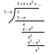 This says $1+x+x^2+…+x^{n-1}$=$\frac {1}{1-x}$
What’s The Function Of $1$-$x$+$x^2$-$x^3$+$x^4$-$x^5$+…?
Let $f(x)$=$1$-$x$+$x^2$-$x^3$+$x^4$-$x^5$+…, then their first, second, third, forth order derivative are below:
$f^{(1)}(x)$=$-1$+$2\cdot x$-$3\cdot x^2$+$4\cdot x^3$-$5\cdot x^4$+…
$f^{(2)}(x)$=$2$-$6\cdot x$+$12\cdot x^2$-$20\cdot x^3$+…
$f^{(3)}(x)$=$-6$+$24\cdot x$-$60\cdot x^2$+…
$f^{(4)}(x)$=$24$-$120\cdot x$+…
Departure from $x$=$0$, where $\triangle x\rightarrow 0$, thus:
$\lim_{\triangle x\rightarrow 0}f(x+\triangle x)$
$\approx\lim_{\triangle x\rightarrow 0}f(\triangle x)$
$=f(0)$+$f^{(1)}(0)\cdot\triangle x$+$\frac {1}{2}\cdot f^{(2)}(0)\cdot(\triangle x)^2$+$\frac {1}{6}\cdot f^{(3)}(0)\cdot(\triangle x)^3$+…
$=1$-$\triangle x$+$(\triangle x)^2$-$(\triangle x)^3$+$(\triangle x)^4$-$(\triangle x)^5$+…
Replace $\triangle x$ by $x$, we finally have $f(x)$
, then:
➀let $f(x)$=$\frac {1}{x}$, then $f(0)$=$\infty$, boom!
➁let $f(x)$=$\frac {1}{x-1}$, then $f(0)$=$-1$, a contradiction!
➂let $f(x)$=$\frac {1}{1-x}$, then:
$f(0)$=$1$
$f^{(1)}(0)$=$-(1-x)^{-2}$=$-1$
$f^{(2)}(0)$=$-2\cdot(1-x)^{-3}$=$-2$, boom!
➃let $f(x)$=$\frac {1}{1+x}$, then:
$f(0)$=$1$
$f^{(1)}(0)$=$-(1+x)^{-2}$=$-1$
$f^{(2)}(0)$=$2\cdot(1+x)^{-3}$=$2$, looks good
$f^{(3)}(0)$=$-6\cdot(1+x)^{-4}$=$-6$, still holds
$f^{(4)}(0)$=$24\cdot(1+x)^{-5}$=$24$, wow, that’s it
Thus, $f(x)$=$\frac {1}{1+x}$ just satisfies this series.
The Integral Of Series
➀by given that $1+x+x^2+…+x^{n-1}$=$\frac {1}{1-x}$, as $n\rightarrow\infty$
Then, $\int 1+x+x^2+…\operatorname dx$=$\int\frac {1}{1-x}\operatorname dx$
$\Rightarrow x+\frac {1}{2}\cdot x^2+\frac {1}{3}\cdot x^3+…$=$-ln(1-x)$
➁by given that $1$-$x$+$x^2$-$x^3$+$x^4$-$x^5$+…+$(x)^{n-1}$=$\frac {1}{1+x}$, as $n\rightarrow\infty$
then, $\int 1-x+x^2-x^3+x^4-x^5+…\operatorname dx$=$\int\frac {1}{1+x}$
$\Rightarrow x-\frac {1}{2}\cdot x^2+\frac {1}{3}\cdot x^3-\frac {1}{4}\cdot x^4+\frac {1}{5}\cdot x^5…$=$ln(1+x)$
➂$\int 1+x+x^2+…\operatorname dx$+$\int 1-x+x^2-x^3+x^4-x^5+…\operatorname dx$
$\;\;$=$x+\frac {1}{2}\cdot x^2+\frac {1}{3}\cdot x^3+…$+$x-\frac {1}{2}\cdot x^2+\frac {1}{3}\cdot x^3…$
$\;\;$=$2\cdot(x+\frac {1}{3}\cdot x^3+\frac {1}{5}\cdot x^5…)$
$\;\;$=$-ln(1-x)$+$ln(1+x)$
$\;\;$=$ln(1+x)$-$ln(1-x)$
$\;\;$=$ln\frac {1+x}{1-x}$…magic
Convergence Test
[1]Definition of partial sum
The partial sum $S_n$ of the series $a_1$+$a_2$+$a_3$+… stops at $a_n$, then the sum of the first n tems is $S_n$=$a_1$+$a_2$+$a_3$+…+$a_n$.
Thus, $S_n$ is part of the total sum.
Ex. the series $\frac {1}{2}$+$\frac {1}{4}$+$\frac {1}{8}$+…has partial sums:
$S_1$=$\frac {1}{2}$,$S_2$=$\frac {3}{4}$,$S_3$=$\frac {7}{8}$,…,$S_n$=$1-\frac {1}{2^n}$
Hence, $\frac {1}{2}$+$\frac {1}{4}$+$\frac {1}{8}$+...converges to $1$, because $S_n\rightarrow 1$, as $a\rightarrow\infty$.
[2]The limit of partial sum
The sum of a series is the limit of its partial sum, for we can have a new idea that $\sum a_n$=$S$, where $S_n\rightarrow S$.
[3]Theorem:
If a series converges($S_n\rightarrow S$), then its terms must approach zero($a_n\rightarrow 0$).
Proof:
By given that $S_n\rightarrow S$, it just converges,
then for $S_{n+1}$ of the $n+1$ terms, $S_{n+1}-S_n\rightarrow 0$ must hold to have $S_{n+1}\rightarrow S_n$, and $S_n\rightarrow S$ by given.
Therefore, the $(n+1)$th term must approaches zero!!
Comparison Test
[1]Comparison test: suppose that $0\le a_n\le b_n$ and $\sum b_n$ converges. Then, $\sum a_n$ converges. A series diverges, if it is above another diverged series.
[2]Comparison test on harmonic series: the harmonic series series $1$+$\frac {1}{2}$+$\frac {1}{3}$+$\frac {1}{4}$+...diverges to infinity.
This section illustrates why by comparing the series with the curve $y$=$\frac {1}{x}$.
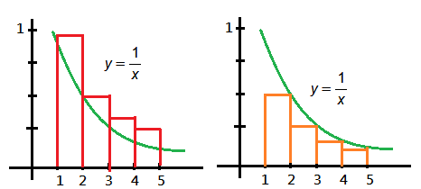 ➀for the rectangle above the curve, each rectangle area $a_n$=$\frac {1}{n}$, then:
$\sum a_n\ge\int_{1}^{n+1}\frac {1}{x}\operatorname dx$=$ln(n+1)$, where $\lim_{n\rightarrow\infty}ln(n+1)$=$\infty$
➁for the area below the curve, we have it that:
$\frac {1}{2}$+$\frac {1}{3}$+$\frac {1}{4}$+…$<\int_{1}^{n}\frac {1}{x}\operatorname dx$=$ln(n)$, $\lim_{n\rightarrow\infty}ln(n)$=$\infty$
The reason we integrate up to $n$ only is due to that each rectangle at $x$ under the curve counts its area in the reciprocal of its next adjacent $x+1$, totally, $n-1$ rectangles.
Then $1$+$\frac {1}{2}$+$\frac {1}{3}$+$\frac {1}{4}$+…$<(1+ln(n))\rightarrow\infty$, as $n\rightarrow\infty$
Put it all together:
$ln(n+1)$<$1$+$\frac {1}{2}$+$\frac {1}{3}$+$\frac {1}{4}$+…<$1+ln(n)$
$\Rightarrow\infty$<$1$+$\frac {1}{2}$+$\frac {1}{3}$+$\frac {1}{4}$+…<$\infty$, as $a\rightarrow\infty$
By squeeze theorem, $1$+$\frac {1}{2}$+$\frac {1}{3}$+$\frac {1}{4}$+…$\rightarrow\infty$, it diverges!!
Integral Test
[1]If $y(x)$ is decreasing, and $y(n)$ agrees with $a_n$, then $a_1$+$a_2$+$a_3$+… and $\int_{0}^{\infty}y(x)\operatorname dx$ both converge or both diverge.
[2]The p-series $\frac {1}{2^p}$+$\frac {1}{3^p}$+$\frac {1}{4^p}$+$\frac {1}{5^p}$+… converges, if $p>1$.
proof:
➀let $y$=$\frac {1}{x^p}$, then $\frac {1}{n^p}$<$\int_{n-1}^{n}\frac {1}{x^p}\operatorname dx$
➁sum it up, we get:
$\sum_{n=2}^{\infty}\frac {1}{n^p}$<$\int_{1}^{\infty}\frac {1}{x^p}\operatorname dx$
$\;\;\;\;$=$\int_{1}^{\infty}x^{-p}\operatorname dx$
$\;\;\;\;$=$\frac {1}{-p+1}\cdot x\vert_1^\infty$
$\;\;\;\;$=$\frac {1}{1-p}\cdot(\infty^{-p+1}-1)$
➂therefore, this series converges, if $p>1$,
hence, $1$+$\sum_{2}^{\infty}\frac {1}{n^p}$<$1$+$\frac {1}{1-p}\cdot(0-1)$=$\frac {p}{p-1}$
Ratio Test Theorem
If $\frac {a_{n+1}}{a_n}$ approaches a limit $L<1$, the series converges.
proof:
There is a hint that we can compare $a_1$+$a_2$+$a_3$+... with $1$+$x$+$x^2$+...
➀choose $L$<$x$<$1$, then we just have:
$\frac {a_{n+1}}{a_n}$<$x$,$\frac {a_{n+2}}{a_{n+1}}$<$x$,$\frac {a_{n+3}}{a_{n+2}}$<$x$,…
➁multiply each inequality, we have:
$\frac {a_{n+1}}{a_n}$<$x$,$\frac {a_{n+2}}{a_{n}}$<$x^2$,$\frac {a_{n+3}}{a_{n}}$<$^3x$,…
$\Rightarrow a_{n+1}<a_{n}\cdot x$,$a_{n+2}<a_{n}\cdot x^2$,$a_{n+3}<a_{n}\cdot x^{3}$,…
$\Rightarrow a_{n+1}$+$a_{n+2}$+$a_{n+3}$+…<$a_n\cdot(x+x^2+x^3+…)$
$\Rightarrow a_{n+1}$+$a_{n+2}$+$a_{n+3}$+…<$a_n\cdot x\cdot(1+x+x^2+…)$
➂since $x$<$1$, compare with the geometric series, $\sum a_n$ just converges.
Root Test Theorem
If the n term in root $(a_n)^{\frac {1}{n}}$ approaches $L$<$1$, the series just converges.
proof:
➀$\lim_{n\rightarrow\infty}(a_n)^{\frac {1}{n}}\rightarrow L<1$…by given
$\Rightarrow(\lim_{n\rightarrow\infty}(a_n)^{\frac {1}{n}})^{n}\rightarrow L^n<1^n$
$\Rightarrow\lim_{n\rightarrow\infty}(a_n)\rightarrow L^n<1$
➁then for the n+1 term, we just have it hold:
$\lim_{n\rightarrow\infty}(a_{n+1})\rightarrow L^{n+1}<1$
➂$\lim_{n\rightarrow\infty}\frac {a_{n+1}}{a_n}\rightarrow\frac {L^{n+1}}{L^{n}}=L<1$, therefore, this series just converges.
Theorem: Limit Comparison Test
If the ratio $\frac {a_n}{b_n}$ approaches a positive limit $L$, then $\sum a_n$,$\sum b_n$ either diverge or converge.
proof:
$\lim_{n\rightarrow\infty}\frac {a_n}{b_n}\rightarrow L>0$…by given
$\Rightarrow\lim_{n\rightarrow\infty}\frac {a_{n+1}}{b_{n+1}}\rightarrow L>0$, also holds
, which implies that $\sum a_n$,$\sum b_n$ are two very closed series, if one converges, another would surely does; for divergence, it is the same.
Convergence Tests: All Series
[1]Definition of absolute convergence:
The series $\sum a_n$ is absolutely convergent, if $\left|\sum a_n\right|$ converges.
Why? This is because changing from $a_n$ to $\left|a_n\right|$ increases the sum. Thus, the smaller $a_n$ is surely to converge, if $\left|\sum a_n\right|$ converges.
[2]Alternating series:
$a_1$-$a_2$+$a_3$-$a_4$+$a_5$-$a_6$+…, in which the signs alternate between plus and minus.
The series $1$-$\frac {1}{2}$+$\frac {1}{3}$-$\frac {1}{4}$+$\frac {1}{5}$-$\frac {1}{6}$+… converges, why?
➀the terms decreasing to zero
➁it decreasing to zero with alternating signs, that is $a_n\rightarrow 0^{+}$,$a_{n+1}\rightarrow 0^{-}$,
hence, $a_n+(-a_{n+1})\rightarrow 0$, where $a_n>a_{n+1}$, the series converges.
[3]An alternating series $a_1$-$a_2$+$a_3$-$a_4$+$a_5$-$a_6$+...converges, if every $a_{n+1}\le a_{n}$ and $a_{n}\rightarrow 0$.
proof::mjtsai1974
➀by given that $a_n\ge a_{n+1}$,$a_n\rightarrow 0$, as $a\rightarrow\infty$, we define $b_i$=$a_i-a_{i+1}$
➁then, $b_n\rightarrow 0$, as $a\rightarrow\infty$ also holds.
➂and $a_n\ge a_{n+1}$ implies that $\frac {a_{n+1}}{a_n}\rightarrow L_a\le 1$, as $n\rightarrow\infty$.
for $L_a=1$, we have $a_n$-$a_{n+1}$=$b_n$=$0$
for $L_a<1$, we have $b_n\rightarrow 0$ also holds.
➃thus, $b_n$ is either zero or decreasing to zero, and $\frac {b_{n+1}}{b_n}\rightarrow L_b$, as $n\rightarrow\infty$, where $L_b\rightarrow 1$ must hold, if $L_a<1$.
Addendum
➀MIT OCW Calculus On-line Textbook by Gilbert Strange
➁MIT OCW Calculus by Gilbert Strange
24 Jan 2018
Prologue To The Exponential Distribution
In probability theory and statistics, the exponential distribution is the model of distribution further developed, base on the most fundamental gamma distribution.
With the basic realization of gamma distributions, we could also treat the exponential distribution a special case of gamma distribution.
It would be greatly helpful in the evaluation of the experimental model build on your hypothesis, the power of test for the precision in the machine learning results.
The Exponential Distribution Illustration
This article would like to guide you through a design of a simple case to generalize the exponential distribution.
➀the experiment is proceeded with the assumption that $x$ is the rate of event occurrence during one time interval $t$, totally, $x\cdot t$ events.
➁suppose $V$ is the volumetric space where these events occur within. Trivially, the success probability of event occurrence, we take it as $P_{success}$=$\frac {x\cdot t}{V}$, then the failure probability could be regarded as $P_{fail}$=$1-\frac {x\cdot t}{V}$.
➂suppose the rate $x$ do exist and remain constant over each disjoint interval for some event occurrence.
➃each disjoint interval are of the same time length, say it $t$, and we further divide it into n subsections. Then each subsection would have $P_{success}$=$\frac {x\cdot t}{V\cdot n}$, then the failure probability could be regarded as $P_{fail}$=$1-\frac {x\cdot t}{V\cdot n}$.
➄we assume that each occurrence of the event in distinct subsection is independent, the success v.s. failure probability in each subsection just matches the the Bernoulli distribution.
➅let the random variable $T$ to be the time it takes until the very first event to occur, and the whole behavior follows the geometric distribution, if it takes time larger than time $t$ for the very first event to occur, then we have such probability:
$P(T>t)$=$\lim_{n\rightarrow\infty}(P_{fail})^{n}$=$\lim_{n\rightarrow\infty}(1-\frac {x\cdot t}{V\cdot n})^{n}$
$(1-\frac {x\cdot t}{V\cdot n})^{n}$
$=C_{0}^{n}1^{n}\cdot(-\frac {x\cdot t}{V\cdot n})^{0}$+$C_{1}^{n}1^{n-1}\cdot(-\frac {x\cdot t}{V\cdot n})^{1}$+$C_{2}^{n}1^{n-2}\cdot(-\frac {x\cdot t}{V\cdot n})^{2}$+…+$C_{n}^{n}1^{0}\cdot(-\frac {x\cdot t}{V\cdot n})^{n}$
Since $\lim_{n\rightarrow\infty}(-\frac {x\cdot t}{V\cdot n})=0$, then:
$P(T>t)$
$=\lim_{n\rightarrow\infty}(1-\frac {x\cdot t}{V\cdot n})^{n}$
$=\lim_{n\rightarrow\infty}1+(-\frac {x\cdot t}{V\cdot n})^{n}$
$\approx\lim_{n\rightarrow\infty}(1+\frac {-x\cdot t}{V\cdot n})^{n}$
Since $e$=$\lim_{n\rightarrow\infty}(1+\frac {1}{n})^{n}$, and
$e^{2}$=$\lim_{n\rightarrow\infty}((1+\frac {1}{n})^{n})^{2}$
$=\lim_{n\rightarrow\infty}((1+\frac {1}{n})^{2})^{n}$
$=\lim_{n\rightarrow\infty}(1+\frac {2}{n}+\frac {1}{n^{2}})^{n}$
$\approx\lim_{n\rightarrow\infty}(1+\frac {2}{n})^{n}$
Then, $P(T>t)$=$e^{-\frac {x\cdot t}{V}}$
➆therefore, $P(T\le t)$=$1-e^{-\frac {x\cdot t}{V}}$, it is the successful probability for events to occur within time $t$.
Above is just the basic illustration of the the exponential distribution. Such scenario would be mostly found in chemical catalyst experiment, or fermentation test in biological laboratory.
Definition Of The Exponential Distribution
Succeeding to the last paragraph, for the simplicity, we take $\lambda$=$\frac {x}{V}$ to be the rate, the intensity. The CDF could be easily defined as below:
$F_{T}(t)$=$1-e^{-\lambda\cdot t}$=$P(T\le t)$
Derivate $F_{T}(t)$ on $t$, we then get its PDF below:
$f_{T}(t)$=$\frac{\operatorname d{F_{T}(t)}}{\operatorname d{t}}$=$\lambda\cdot e^{-\lambda\cdot t}$
To validate it,
$P(T\le a)$
$=\int_{0}^{a}\lambda\cdot e^{-\lambda\cdot t}\operatorname dt$
$=-e^{-\lambda\cdot t}\vert_{0}^{a}$
$=1-e^{-\lambda\cdot a}$, take $t$=$a$
Relationship With The Gamma Distribution
Be recalled that the PDF of the gamma distribution:
$f_{X}(x)=\frac {1}{\beta^{\alpha}\cdot\Gamma(\alpha)}\cdot x^{\alpha-1}\cdot e^{-\frac{x}{\beta}}$
Take $\alpha$=$1$, $\lambda$=$\frac {1}{\beta}$, you can easily find that the exponential distribution a special case of gamma distribution. Change $X$ to $T$, $x$ to $t$, they are exactly the same thing!!!
Below chart exhibits its PDF with regards to $\lambda$ set to $0.5$,$0.333$:
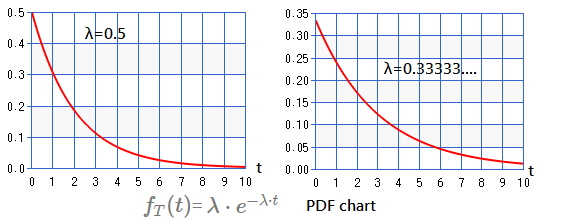 Next chart illustrate the cumulative distribution with $\lambda$ set to $0.5$,$0.333$:
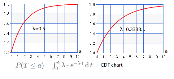
Moments Of The Exponential Distribution
The most efficient way to get the expect value and variance would be the moments.
➀take $\alpha$=$1$, $\lambda$=$\frac {1}{\beta}$, we will have the moments below:
$\mu_{r}$=$E\lbrack X^{r}\rbrack$=$\frac {1}{\beta}\int_{0}^{\infty}x^{r}\cdot e^{-\frac {x}{\beta}}\operatorname dx$
➁let $y$=$\frac {x}{\beta}$, $\operatorname dy$=$\frac {1}{\beta}\cdot\operatorname dx$, then:
$\mu_{r}$=$\frac {1}{\beta}\int_{0}^{\infty}(\beta\cdot y)^{r}\cdot e^{-y}\cdot\beta\cdot\operatorname dy$
$\;\;\;\;$=$\beta^{r}\int_{0}^{\infty}(y)^{r}\cdot e^{-y}\operatorname dy$
$\;\;\;\;$=$\beta^{r}\cdot\Gamma(r+1)$
Therefore, we have $\mu_1$=$\beta\cdot\Gamma(2)$=$\beta$
And $\mu_2$=$\beta^{2}\cdot\Gamma(3)$=$\beta^{2}\cdot 2\cdot\Gamma(2)$=$2\cdot\beta^{2}$
Finally, the expect value $\mu_{1}$=$E\lbrack X\rbrack$=$\beta$
The variance $Var\lbrack X\rbrack$=$E\lbrack X^2\rbrack$-$E^2\lbrack X\rbrack$=$\beta^{2}$
Recall that we take $\lambda$=$\frac {1}{\beta}$, hence, $E\lbrack X\rbrack$=$\frac {1}{\lambda}$, $Var\lbrack X\rbrack$=$(\frac {1}{\lambda})^2$
16 Jan 2018
Prologue To The Beta Distribution
In probability theory and statistics, base on the most fundamental gamma distribution, beta distribution is one of the many models of distributions further developed.
With the basic realization of gamma distributions, we could also treat the beta function a special combination of gamma functions.
The beta function is important in calculus and analysis due to its close connection to the gamma function, which is itself a generalization of the factorial function, and would be greatly
helpful in the evaluation, the power of test for the regression model build on your hypothesis, the precision in the machine learning results.
Begin From The Beta Function
The beta function, also known as Euler’s integral of the first kind. We formulate the beta function in below two expressions:
$\beta(x,y)$=$\int_{0}^{\infty}t^{x-1}\cdot(1+t)^{-x-y}\operatorname dt$…(1);
$\beta(x,y)$=$\int_{0}^{1}t^{x-1}\cdot(1-t)^{y-1}\operatorname dt$…(2);
Where (1)=(2), next to prove it.
proof:
➀to change from $\int_{0}^{\infty}$ to $\int_{0}^{1}$, we focus on $t$:
$\int_{0}^{\infty}t^{x-1}\cdot(1+t)^{-x-y}\operatorname dt$
$=\int_{0}^{\infty}t^{x-1}\cdot(\frac {1}{1+t})^{x+y}\operatorname dt$
$=\int_{0}^{\infty}(\frac {t}{1+t})^{x-1}\cdot(\frac {1}{1+t})^{y+1}\operatorname dt$
➁take $w$=$\frac {t}{1+t}$, then $1-w$=$\frac {1}{1+t}$
$w$=$1-\frac {1}{1+t}$=$1-(1+t)^{-1}$
$\Rightarrow\frac {\operatorname dw}{\operatorname dt}$=$(\frac {1}{1+t})^{2}$
$\Rightarrow \operatorname dw$=$(\frac {1}{1+t})^{2}\cdot\operatorname dt$=$(1+t)^{-2}\cdot\operatorname dt$
$\Rightarrow \operatorname dt$=$(1+t)^{2}\cdot\operatorname dw$
➂$\lim_{t\rightarrow\infty}\frac t{1+t}=1$, therefore $\int_{0}^{\infty}\operatorname dt$ transforms to $\int_{0}^{1}\operatorname dw$ is reasonable, it says that integration from $0$ to $\infty$ could be changed to integration from $0$ to $1$.
$\int_{0}^{\infty}(\frac {t}{1+t})^{x-1}\cdot(\frac {1}{1+t})^{y+1}\operatorname dt$
$=\int_{0}^{1}w^{x-1}\cdot(1-w)^{y+1}\cdot(1+t)^{2}\operatorname dw$
, where $1-w$=$(1+t)^{-1}$, and we have it that:
$(1+t)^{2}$=$((1+t)^{-1})^{-2}$=$(1-w)^{-2}$
therefore,
$=\int_{0}^{1}w^{x-1}\cdot(1-w)^{y+1}\cdot(1-w)^{-2}\operatorname dw$
$=\int_{0}^{1}w^{x-1}\cdot(1-w)^{y-1}\operatorname dw$
In some textbooks or web articles, they intend to use the form:
$\beta(x,y)$=$\int_{0}^{1}t^{x}\cdot(1-t)^{y}\operatorname dt$
The tiny difference mainly in the input parameters, $x\ge 1$, $y\ge 1$.
The Definition Of The Beta Function
Next come to visit the definition of the beta function.
$\beta(x,y)$=$\frac {\Gamma(x)\cdot\Gamma(y)}{\Gamma(x+y)}$…by definition
proof:
➀
$\Gamma(x)\cdot\Gamma(y)$
$=\int_{0}^{\infty}u^{x-1}\cdot e^{-u}\operatorname du\cdot\int_{0}^{\infty}v^{y-1}\cdot e^{-v}\operatorname dv$
$=\int_{0}^{\infty}\int_{0}^{\infty}u^{x-1}\cdot v^{y-1}\cdot e^{-u-v}\operatorname du\operatorname dv$
➁take $u$=$v\cdot t$, then $\operatorname du$=$v\cdot\operatorname dt$
why? Because gamma function focus on the parameter of power, not integral itself. Expand from ➀:
$\int_{0}^{\infty}\int_{0}^{\infty}u^{x-1}\cdot v^{y-1}\cdot e^{-(u+v)}\operatorname du\operatorname dv$
$=\int_{0}^{\infty}\int_{0}^{\infty}v\cdot (v\cdot t)^{x-1}\cdot v^{y-1}\cdot e^{-(v\cdot t+v)}\operatorname dt\operatorname dv$
$=\int_{0}^{\infty}\int_{0}^{\infty}t^{x-1}\cdot v^{x+y-1}\cdot e^{-(v\cdot t+v)}\operatorname dt\operatorname dv$
➂take $w$=$v\cdot t+v$, then we have:
$v$=$\frac {w}{1+t}$, $\operatorname dv$=$\frac {1}{1+t}\cdot\operatorname dw$
$\int_{0}^{\infty}\int_{0}^{\infty}t^{x-1}\cdot v^{x+y-1}\cdot e^{-(v\cdot t+v)}\operatorname dt\operatorname dv$
$=\int_{0}^{\infty}\int_{0}^{\infty}t^{x-1}\cdot (\frac {w}{1+t})^{x+y-1}\cdot e^{-w}\operatorname dt\frac {1}{1+t}\cdot\operatorname dw$
$=\int_{0}^{\infty}\int_{0}^{\infty}t^{x-1}\cdot (\frac {1}{1+t})^{x+y}\cdot w^{(x+y-1)}\cdot e^{-w}\operatorname dt\operatorname dw$
$=\int_{0}^{\infty}w^{(x+y-1)}\cdot e^{-w}\operatorname dw\cdot\int_{0}^{\infty}t^{x-1}\cdot(\frac {1}{1+t})^{x+y}\operatorname dt$
$=\Gamma(x+y)\cdot\int_{0}^{\infty}t^{x-1}\cdot (1+t)^{-x-y}\operatorname dt$
$=\Gamma(x+y)\cdot\beta(x,y)$
Finally, we just have it proved:
$\Gamma(x)\cdot\Gamma(y)$
$=\Gamma(x+y)\cdot\int_{0}^{\infty}t^{x-1}\cdot (1+t)^{-x-y}\operatorname dt$
$=\Gamma(x+y)\cdot\beta(x,y)$
$\Rightarrow\beta(x,y)=\frac {\Gamma(x)\cdot\Gamma(y)}{\Gamma(x+y)}$
Symmetry Of The Beta Function
$\beta(x,y)$=$\beta(y,x)$…$\beta$ is symmetric.
proof:
➀begin by definition,
$\beta(x,y)$=$\int_{0}^{1}t^{x-1}\cdot(1-t)^{y-1}\operatorname dt$
➁take $v$=$1-t$, then $t$=$1-v$
therefore, $\operatorname dv$=$-\operatorname dt$, $\operatorname dt$=$-\operatorname dv$
and $0\le t\le 1$, $-1\le -v\le 0$
➂expand from beta function:
$\beta(x,y)$
$=\int_{0}^{1}t^{x-1}\cdot(1-t)^{y-1}\operatorname dt$
$=\int_{-1}^{0}(1-v)^{x-1}\cdot(v)^{y-1}(\operatorname -dv)$
$=\int_{-1}^{0}(1-v)^{x-1}\cdot(v)^{y-1}\operatorname d(-v)$…$\operatorname -dv=\operatorname d(-v)$
$=\int_{0}^{1}(1-v)^{x-1}\cdot(v)^{y-1}\operatorname dv$
$=\beta(y,x)$
$\beta$ function is symmetric
is thus proved.
The Beta Distribution PDF
For $0<x<1$ and $X$ is a random variable of beta distribution, where $x\in X$, the PDF of beta distribution is defined below:
$f_{X}(x)$=$\frac {1}{\beta(a,b)}\cdot x^{a-1}\cdot(1-x)^{b-1}$
Caution must be made that $f_{X}(x)=0$ for the case $x\not\in [0,1]$. Next we go to prove it.
proof:
➀departure from integrating its PDF from negative to positive infinity.
$\int_{-\infty}^{\infty}f_{X}(x)\operatorname dx$
$=\int_{-\infty}^{\infty}\frac {1}{\beta(a,b)}\cdot x^{a-1}\cdot(1-x)^{b-1}\operatorname dx$
$=\frac {1}{\beta(a,b)}\int_{-\infty}^{\infty}x^{a-1}\cdot(1-x)^{b-1}\operatorname dx$
➁suppose the definition of its PDF is true, we can integrate, ranging from $0$ to $1$:
$\frac {1}{\beta(a,b)}\int_{0}^{1}x^{a-1}\cdot(1-x)^{b-1}\operatorname dx$
$=\frac {1}{\beta(a,b)}\cdot\beta(a,b)$
$=1$
Be recalled that $f_{X}(x)=0$ for the case $x\not\in [0,1]$
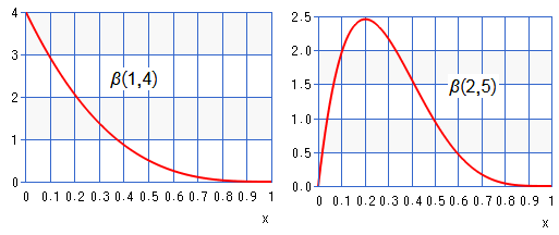
Below we exhibit the PDF of $\beta(1,4)$, $\beta(2,5)$:
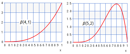
 Then exhibit the PDF of $\beta(4,1)$, $\beta(5,2)$:
 Finally, the exhibition of PDF of $\beta(2,2)$, $\beta(4,4)$:
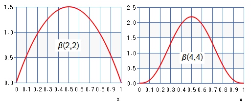 You can find it more approximate normal distribution for we input parameters with $a=b$, and the graph would be right skew for $a<b$, and left skew for $a>b$.
The Beta Distribution CDF
The CDF of beta distribution is defined below:
$F_{X}(k)$=$\frac {\beta(k,a,b)}{\beta(a,b)}$=$\frac {\int_{0}^{k}x^{a-1}\cdot(1-x)^{b-1}}{\beta(a,b)}$
proof:
$F_{X}(k)$
$=\int_{-\infty}^{k}f_X(x)\operatorname dx$
$=\int_{0}^{k}\frac {1}{\beta(a,b)}\cdot x^{a-1}\cdot(1-x)^{b-1}\operatorname dx$
$=\frac {1}{\beta(a,b)}\int_{0}^{k}x^{a-1}\cdot(1-x)^{b-1}\operatorname dx$
, where we take $\beta(k,a,b)$=$\int_{0}^{k}x^{a-1}\cdot(1-x)^{b-1}\operatorname dx$
In general, two CDFs could be further defined:
➀lower CDF, $\frac {\int_{0}^{k}x^{a-1}\cdot(1-x)^{b-1}}{\beta(a,b)}$, where $k\le 1$.
➁upper CDF, $\frac {\int_{k}^{1}x^{a-1}\cdot(1-x)^{b-1}}{\beta(a,b)}$
Expect Value Of The Beta Distribution
For any valid random variable X of beta distribution, the expect value is given:
$E\lbrack X\rbrack$=$\frac {a}{a+b}$
proof:
$E\lbrack X\rbrack$
$=\int_{0}^{\infty}x\cdot\frac {1}{\beta(a,b)}\cdot x^{a-1}\cdot(1-x)^{b-1}\operatorname dx$
$=\frac {1}{\beta(a,b)}\cdot\int_{0}^{\infty}x^{a}\cdot(1-x)^{b-1}\operatorname dx$
$=(\frac {\Gamma(a)\cdot\Gamma(b)}{\Gamma(a+b)})^{-1}\cdot\beta(a+1,b)$
$=\frac {\Gamma(a+b)}{\Gamma(a)\cdot\Gamma(b)}\cdot\frac {\Gamma(a+1)\cdot\Gamma(b)}{\Gamma(a+b+1)}$
$=\frac {\Gamma(a+b)}{\Gamma(a)\cdot\Gamma(b)}\cdot\frac {a\cdot\Gamma(a)\cdot\Gamma(b)}{(a+b)\cdot\Gamma(a+b)}$
$=\frac {a}{a+b}$
Variance Of The Beta Distribution
For any valid random variable X of beta distribution, the variance is given:
$Var\lbrack X\rbrack$=$\frac {a\cdot b}{(a+b+1)\cdot(a+b)^{2}}$
proof:
$Var\lbrack X\rbrack$=$E\lbrack X^{2}\rbrack$-$E^{2}\lbrack X\rbrack$, to figure out the variance, the term $E\lbrack X^{2}\rbrack$ should be come out.
$E\lbrack X^{2}\rbrack$
$=\int_{0}^{\infty}x^{2}\cdot\frac {1}{\beta(a,b)}\cdot x^{a-1}\cdot(1-x)^{b-1}\operatorname dx$
$=\int_{0}^{\infty}\frac {1}{\beta(a,b)}\cdot x^{a+1}\cdot(1-x)^{b-1}\operatorname dx$
$=\frac {1}{\beta(a,b)}\cdot\int_{0}^{\infty}x^{a+1}\cdot(1-x)^{b-1}\operatorname dx$
$=\frac {1}{\beta(a,b)}\cdot\beta(a+2,b)$
$Var\lbrack X\rbrack$
$=\frac {1}{\beta(a,b)}\cdot\beta(a+2,b)$-$(\frac {a}{a+b})^{2}$
…after deduction…
$=\frac {a\cdot b}{(a+b+1)\cdot(a+b)^{2}}$
k-th Moment Of Beta Random Variable
$\mu_{k}$
$=E\lbrack X^{k}\rbrack$
$=\frac {\beta(a+k,b)}{\beta(a,b)}$
$={\textstyle\prod_{n=0}^{k-1}}\frac{a+n}{a+b+n}$
proof:
$E\lbrack X^{k}\rbrack$
$=\int_{0}^{\infty}x^{k}\cdot\frac {1}{\beta(a,b)}\cdot x^{a-1}\cdot(1-x)^{b-1}\operatorname dx$
$=\frac {1}{\beta(a,b)}\cdot\int_{0}^{\infty}x^{a+k-1}\cdot(1-x)^{b-1}\operatorname dx$
$=\frac {\Gamma(a+b)}{\Gamma(a)\cdot\Gamma(b)}\cdot\frac {\Gamma(a+k)\cdot\Gamma(b)}{\Gamma(a+b+k)}$
$=\frac {\Gamma(a+b)}{\Gamma(a)\cdot\Gamma(b)}\cdot\frac {(a+k-1)\cdot(a+k-2)…a\cdot\Gamma(a)\cdot\Gamma(b)}{(a+b+k-1)\cdot(a+b+k-2)…(a+b)\cdot\Gamma(a+b)}$
$=\frac {a\cdot(a+1)\cdot(a+2)…(a+k-2)\cdot(a+k-1)}{(a+b)\cdot(a+b+1)…(a+b+k-2)\cdot(a+b+k-1)}$
$={\textstyle\prod_{n=0}^{k-1}}\frac{a+n}{a+b+n}$
Where $X$ is any beta random variable, $x\in X$.
Moment Generating Function Of Beta Random Variable
$M_{X}(t)$
$=\sum_{k=0}^{\infty}\frac {t^{k}}{k!}\cdot\frac {\beta(a+k,b)}{\beta(a,b)}$
$=1+\sum_{k=1}^{\infty}\frac {t^{k}}{k!}\cdot\frac {\beta(a+k,b)}{\beta(a,b)}$
proof:
$M_{X}(t)$
$=\int_{0}^{1}e^{x\cdot t}\cdot\frac {x^{a-1}\cdot(1-x)^{b-1}}{\beta(a,b)}\operatorname dx$…MGF’s definition
$=\frac {1}{\beta(a,b)}\cdot\int_{0}^{1}e^{x\cdot t}\cdot x^{a-1}\cdot(1-x)^{b-1}\operatorname dx$
$=\frac {1}{\beta(a,b)}\cdot\int_{0}^{1}(\sum_{k=0}^{\infty}\frac {(x\cdot t)^{k}}{k!})\cdot x^{a-1}\cdot(1-x)^{b-1}\operatorname dx$
$=\frac {1}{\beta(a,b)}\cdot\sum_{k=0}^{\infty}\int_{0}^{1}\frac {(x\cdot t)^{k}}{k!}\cdot x^{a-1}\cdot(1-x)^{b-1}\operatorname dx$
$=\frac {1}{\beta(a,b)}\cdot\sum_{k=0}^{\infty}\frac {t^{k}}{k!}\int_{0}^{1}x^{k}\cdot x^{a-1}\cdot(1-x)^{b-1}\operatorname dx$
$=\frac {1}{\beta(a,b)}\cdot\sum_{k=0}^{\infty}\frac {t^{k}}{k!}\int_{0}^{1}x^{a+k-1}\cdot(1-x)^{b-1}\operatorname dx$
$=\frac {1}{\beta(a,b)}\cdot\sum_{k=0}^{\infty}\frac {t^{k}}{k!}\cdot\beta(a+k,b)$
$=\sum_{k=0}^{\infty}\frac {t^{k}}{k!}\frac {beta(a+k,b)}{\beta(a,b)}$
$=1+\sum_{k=1}^{\infty}\frac {t^{k}}{k!}\cdot\mu_{k}$
$=1+\sum_{k=1}^{\infty}\frac {t^{k}}{k!}\cdot E\lbrack X^{k}\rbrack$
$=1+\sum_{k=1}^{\infty}\frac {t^{k}}{k!}\cdot{\textstyle\prod_{n=0}^{k-1}}\frac{a+n}{a+b+n}$
Where $X$ is any beta random variable, $x\in X$.
15 Jan 2018
Prologue To The t Distribution
In probability theory and statistics, base on the most fundamental gamma distribution, t distribution is one of the many models of distributions further developed, furthermore, its definition is based on the central limit theorem.
With the basic realization of gamma, chi-square distributions, we could also treat the t distribution a special joint case of standard normal distribution and the chi-square distribution.
It would be greatly helpful in the evaluation of the regression model build on your hypothesis, the power of test for the precision in the machine learning results.
Why Do We Need The t Distribution?
As we know that $\frac {\overline {X_n}-\mu}{\sigma/\sqrt n}\sim ɸ(0,1)$, by the central limit theorem, when $n\rightarrow\infty$, the term $\frac {\overline {X_n}-\mu}{S/\sqrt n}$ approximates $\frac {\overline {X_n}-\mu}{\sigma/\sqrt n}$, where
➀$S$ is the sample deviation.
➁$\sigma$ is the population deviation.
After experiments over so many years, statisticians have it that when sample size is less than 30, $\frac {\overline {X_n}-\mu}{S/\sqrt n}\not\sim ɸ(0,1)$ as a conclusion, for $n<30$, it would be insufficient the quantity of sample size to be distributed in normal distribution.
That’s why we need to have t distribution, by usual, we take $T$=$\frac {\overline {X_n}-\mu}{S/\sqrt n}$.
Expand The Definition Of The t Distribution
Let T to be a random variable, expand from where it is defined:
$T$=$\frac {\overline {X_n}-\mu}{S/\sqrt n}$
$\;\;$=$\frac {\overline {X_n}-\mu}{\sigma/\sqrt n}$/$\frac {S/\sqrt n}{\sigma/\sqrt n}$
$\;\;$=$\frac {Z}{S/\sigma}$, where $Z\sim ɸ(0,1)$
$\;\;$=$\frac {Z}{\sqrt {S^2/\sigma^2}}$
$\;\;$=$\frac {Z}{\sqrt {\frac {\chi_{n-1}^2}{n-1}}}$
, where we have:
➀$\chi_{n-1}^2$=$(n-1)\cdot S^2$/$\sigma^2$
➁$n-1$ is the degree of freedom.
The t Distribution PDF
The PDF of t distribution is given by:
$f_{T}(t)$=$\frac {\Gamma(\frac {\nu+1}{2})}{\sqrt {\pi\cdot\nu}\cdot\Gamma(\frac {\nu}{2})}\cdot(1+\frac {t^2}{\nu})^{-\frac {\nu+1}{2}}$,
where $\nu$ is the degree of freedom, $-\infty<t<\infty$.
proof:
➀please recall that $T$=$\frac {Z}{\sqrt {\frac {\chi_{n-1}^2}{n-1}}}$, and we learn the deduction of the F distribution joint PDF.
Take $f_Z(z)$=$\frac {1}{\sqrt {2\cdot\pi}}\cdot e^{-\frac {z^2}{2}}$, where $-\infty<z<\infty$, $Z\sim ɸ(0,1)$.
Take $f_{\chi_{\nu}^2}(x)$=$\frac {x^{\frac {\nu}{2}-1}}{2^{\frac {\nu}{2}}\cdot\Gamma(\frac {\nu}{2})}\cdot e^{-\frac {x}{2}}$, where $0<x<\infty$, $X \sim\chi_{\nu}^2$.
➁express the joint PDF in below form:
$f_{Z,\chi_{\nu}^2}(z,x)$=$f_Z(z)\cdot f_{\chi_{\nu}^2}(x)$, where $z\in Z$, $x\in X$
$\Rightarrow F_{Z,\chi_{\nu}^2}(z,x)$=$\int_{-\infty}^{\infty}\int_{0}^{\infty}f_Z(z)\cdot f_{X}(x)\operatorname dx\operatorname dz$
For the simplicity of notation, we use $f_{X}(x)$ for $f_{\chi_{\nu}^2}(x)$, since $X \sim\chi_{\nu}^2$, and the $F_{Z,\chi_{\nu}^2}(z,x)$ is the CDF(cumulative distributed function).
➂by the definition of $T$=$\frac {Z}{\sqrt {\frac {\chi_{n-1}^2}{n-1}}}$
Let $t$=$z$/$\sqrt\frac {x}{\nu}$, and, why we use $x$, not $x^2$?
Be noted that $x$ is one sample distributed in $\chi_{\nu}^2$. Don’t get confused!!
➃let $z$=$\frac {t\cdot\sqrt x}{\sqrt \nu}$, $\operatorname dz$=$\frac {\sqrt x}{\sqrt \nu}\cdot\operatorname dt$
We can express $z$ in terms of $t$, which then in turns expressed in terms of $x$.
$F_{Z,\chi_{\nu}^2}(z,x)$
$=F_{T,\chi_{\nu}^2}(t,x)$, where $t \in T$
$=\int_{-\infty}^{\infty}\int_{0}^{\infty}f_Z(\frac {t\cdot\sqrt x}{\sqrt \nu})\cdot f_{X}(x)\operatorname dx\frac {\sqrt x}{\sqrt \nu}\cdot\operatorname dt$
$=\int_{-\infty}^{\infty}\int_{0}^{\infty}\frac {1}{\sqrt {2\cdot\pi}}\cdot e^{-\frac {t^2}{2}\cdot\frac {x}{\nu}}\cdot\frac {x^{\frac {\nu}{2}-1}\cdot e^{-\frac {x}{2}}}{2^{\frac {\nu}{2}}\cdot\Gamma(\frac {\nu}{2})}\operatorname dx\frac {\sqrt x}{\sqrt \nu}\cdot\operatorname dt$
$=\frac {1}{\sqrt {2\cdot\pi}\cdot\sqrt\nu}\cdot\frac {1}{2^{\frac {\nu}{2}}\cdot\Gamma(\frac {\nu}{2})}\int_{-\infty}^{\infty}\int_{0}^{\infty}x^{\frac {\nu+1}{2}-1}\cdot e^{-(\frac {t^2}{2}\cdot\frac {x}{\nu}+\frac {x}{2})}\operatorname dx\operatorname dt$
➄let $w$=$\frac {t^2}{2}\cdot\frac {x}{\nu}+\frac {x}{2}$=$\frac {(t^2+\nu)\cdot x}{2\cdot\nu}$
, then $\operatorname dw$=$\frac {t^2+\nu}{2\cdot\nu}\cdot\operatorname dx$
, and $x$=$\frac {2\cdot\nu}{t^2+\nu}\cdot w$
, therefore $\operatorname dx$=$\frac {2\cdot\nu}{t^2+\nu}\cdot\operatorname dw$
$F_{T,\chi_{\nu}^2}(t,x)$
$=\frac {1}{\sqrt {2\cdot\pi}\cdot\sqrt\nu}\cdot\frac {1}{2^{\frac {\nu}{2}}\cdot\Gamma(\frac {\nu}{2})}\int_{-\infty}^{\infty}\int_{0}^{\infty}(\frac {2\cdot\nu}{t^2+\nu}\cdot w)^{\frac {\nu+1}{2}-1}\cdot e^{-w}\cdot\frac {2\cdot\nu}{t^2+\nu}\cdot\operatorname dw\operatorname dt$
$=\frac {1}{\sqrt {2\cdot\pi}\cdot\sqrt\nu}\cdot\frac {1}{2^{\frac {\nu}{2}}\cdot\Gamma(\frac {\nu}{2})}\cdot\Gamma(\frac {\nu+1}{2})\int_{-\infty}^{\infty}(\frac {2\cdot\nu}{t^2+\nu})^{\frac {\nu+1}{2}}\operatorname dt$
, where $\Gamma(\frac {\nu+1}{2})$=$\int_{0}^{\infty}e^{-w}\cdot w^{\frac {\nu+1}{2}-1}\operatorname dw$
$=\frac {1}{\sqrt {2\cdot\pi}\cdot\sqrt\nu}\cdot\frac {1}{2^{\frac {\nu}{2}}\cdot\Gamma(\frac {\nu}{2})}\cdot\Gamma(\frac {\nu+1}{2})\int_{-\infty}^{\infty}(\frac {t^2+\nu}{2\cdot\nu})^{-\frac {\nu+1}{2}}\operatorname dt$
➅simplify the notation from $F_{T,\chi_{\nu}^2}(t,x)$ to $F_{T}(t)$, then:
$F_{T,\chi_{\nu}^2}(t,x)$
$=F_{T}(t)$
$=\frac {1}{\sqrt {2\cdot\pi}\cdot\sqrt\nu}\cdot\frac {1}{2^{\frac {\nu}{2}}\cdot\Gamma(\frac {\nu}{2})}\cdot\Gamma(\frac {\nu+1}{2})\int_{-\infty}^{\infty}(\frac {t^2+\nu}{2\cdot\nu})^{-\frac {\nu+1}{2}}\operatorname dt$
$f_{T}(t)$=$\frac {\operatorname dF_{T}(t)}{\operatorname dt}$
$=\frac {1}{\sqrt {2\cdot\pi}\cdot\sqrt\nu}\cdot\frac {1}{2^{\frac {\nu}{2}}\cdot\Gamma(\frac {\nu}{2})}\cdot\Gamma(\frac {\nu+1}{2})\cdot (\frac {t^2+\nu}{2\cdot\nu})^{-\frac {\nu+1}{2}}$
After the deduction, we finally have it that:
$f_{T}(t)$=$\frac {\Gamma(\frac {\nu+1}{2})}{\sqrt {\pi\cdot\nu}\cdot\Gamma(\frac {\nu}{2})}\cdot(1+\frac {t^2}{\nu})^{-\frac {\nu+1}{2}}$
Moments Of The t Distribution
Begin from PDF of t distribution, we’d like to further regularize it:
$f_{T}(t)$
$=\frac {\Gamma(\frac {\nu+1}{2})}{\sqrt {\pi\cdot\nu}\cdot\Gamma(\frac {\nu}{2})}\cdot(1+\frac {t^2}{\nu})^{-\frac {\nu+1}{2}}$
$=\frac {1}{\sqrt\nu}\cdot\frac {\Gamma(\frac {\nu}{2}+\frac {1}{2})}{\Gamma(\frac {\nu}{2})\cdot\Gamma(\frac {1}{2})}\cdot(1+\frac {t^2}{\nu})^{-\frac {\nu+1}{2}}$
$=\frac {1}{\sqrt\nu}\cdot\frac {1}{\beta(\frac {\nu}{2},\frac {1}{2})}\cdot(1+\frac {t^2}{\nu})^{-\frac {\nu+1}{2}}$
, where $\sqrt\pi$=$\Gamma(\frac {1}{2})$, $\frac {\Gamma(\frac {\nu}{2}+\frac {1}{2})}{\Gamma(\frac {\nu}{2})\cdot\Gamma(\frac {1}{2})}$=$\beta(\frac {\nu}{2},\frac {1}{2})^{-1}$
The moments would be a cofactor in the expect value and variance of the t distribution.
For any $t\in T$, where $T$ is a random variable in t distribution. The k-th ordinary moment would be:
$E_{k}\lbrack t\rbrack$
$=\frac {1}{\sqrt\nu}\cdot\frac {1}{\beta(\frac {\nu}{2},\frac {1}{2})}\int_{-\infty}^{\infty}t^{k}\cdot(1+\frac {t^2}{\nu})^{-\frac {\nu+1}{2}}\operatorname dt$
$=\frac {1}{\sqrt\nu}\cdot\frac {1}{\beta(\frac {\nu}{2},\frac {1}{2})}\cdot(\int_{-\infty}^{0}t^{k}\cdot(1+\frac {t^2}{\nu})^{-\frac {\nu+1}{2}}\operatorname dt$+$\int_{0}^{\infty}t^{k}\cdot(1+\frac {t^2}{\nu})^{-\frac {\nu+1}{2}}\operatorname dt)$
Expect Value Of The t Distribution
It’s the case when $k=1$:
$\int_{-\infty}^{0}t^{1}\cdot(1+\frac {t^2}{\nu})^{-\frac {\nu+1}{2}}\operatorname dt$=$-\int_{0}^{\infty}t^{1}\cdot(1+\frac {t^2}{\nu})^{-\frac {\nu+1}{2}}\operatorname dt$
When $k=1$, integrate from negative infinity to $0$, is equivalent to negate the integration from $0$ to the infinity.
Therefore, $\mu_{1}$=$E\lbrack t\rbrack$=$0$, the expect value is $0$.
Variance Of The t Distribution
➀the variance involves the 2nd order moment, it is the case when $k=2$, integrate from negative infinity to $0$, is equivalent to the integration from $0$ to the infinity. Therefore, we have it that:
$\mu_{2}$=$E_{2}\lbrack t\rbrack$
$=E\lbrack t^{2}\rbrack$
$=\frac {1}{\sqrt\nu}\cdot\frac {1}{\beta(\frac {\nu}{2},\frac {1}{2})}\cdot 2\cdot\int_{0}^{\infty}t^{2}\cdot(1+\frac {t^2}{\nu})^{-\frac {\nu+1}{2}}\operatorname dt$
➁take $w$=$\frac {t^{2}}{\nu}$, then $t$=$\sqrt w\cdot\nu$
, and $\operatorname dw$=$\frac {2\cdot t}{\nu}\cdot\operatorname dt$, $\operatorname dt$=$\frac {\nu}{2\cdot t}\cdot\operatorname dw$
➂expand from the 2nd order moment:
$E_{2}\lbrack t\rbrack$
$=\frac {1}{\sqrt\nu}\cdot\frac {1}{\beta(\frac {\nu}{2},\frac {1}{2})}\cdot 2\cdot\int_{0}^{\infty}\frac {\nu}{2\cdot t}\cdot t^{2}\cdot(1+w)^{-\frac {\nu+1}{2}}\operatorname dw$
$=\frac {1}{\sqrt\nu}\cdot\frac {1}{\beta(\frac {\nu}{2},\frac {1}{2})}\cdot 2\cdot\int_{0}^{\infty}\frac {\nu}{2}\cdot(w\cdot\nu)^{\frac {1}{2}}\cdot(1+w)^{-\frac {\nu+1}{2}}\operatorname dw$
$=\frac {1}{\sqrt\nu}\cdot\frac {1}{\beta(\frac {\nu}{2},\frac {1}{2})}\cdot 2\cdot\frac {(\nu)^{\frac {3}{2}}}{2}\int_{0}^{\infty}(w)^{\frac {1}{2}}\cdot(1+w)^{-\frac {\nu+1}{2}}\operatorname dw$
➃investigate the power term of $w$, $1+w$, they could be refined:
$\frac {1}{2}$=$\frac {3}{2}-1$, $-\frac {\nu+1}{2}$=$-\frac {3}{2}-\frac {\nu-2}{2}$
➄continue above equality:
$=\frac {1}{\sqrt\nu}\cdot\frac {1}{\beta(\frac {\nu}{2},\frac {1}{2})}\cdot(\nu)^{\frac {3}{2}}\cdot\beta(\frac {3}{2},\frac {\nu-2}{2})$
$=\nu\cdot\frac {\Gamma(\frac {\nu}{2}+\frac {1}{2})}{\Gamma(\frac {\nu}{2})\cdot\Gamma(\frac {1}{2})}\cdot\frac {\Gamma(\frac {3}{2})\cdot\Gamma(\frac {\nu-2}{2})}{\Gamma(\frac {3}{2}+\frac {\nu-2}{2})}$
➅further simplify below terms:
$\Gamma(\frac {3}{2})$=$\frac {1}{2}\cdot\Gamma(\frac {1}{2})$,
$\Gamma(\frac {3}{2}+\frac {\nu-2}{2})$=$\Gamma(\frac {\nu}{2}+\frac {1}{2})$, and,
As to $\Gamma(\frac {\nu-2}{2})$, begin by $\Gamma(\frac {\nu}{2})$:
$\Gamma(\frac {\nu}{2})$=$\frac {\nu-2}{2}\cdot\Gamma(\frac {\nu}{2}-1)$
thus, $\Gamma(\frac {\nu-2}{2})$=$\frac {2}{\nu-2}\cdot\Gamma(\frac {\nu}{2})$
➆put it all together:
$E_{2}\lbrack t\rbrack$
$=\nu\cdot\frac {\Gamma(\frac {\nu}{2}+\frac {1}{2})}{\Gamma(\frac {\nu}{2})\cdot\Gamma(\frac {1}{2})}\cdot\frac {\frac {1}{2}\cdot\Gamma(\frac {1}{2})\cdot\frac {2}{\nu-2}\cdot\Gamma(\frac {\nu}{2})}{\Gamma(\frac {\nu}{2}+\frac {1}{2})}$
$=\frac {\nu}{\nu-2}$
Finally, we can deduce it out the variance:
$Var\lbrack t\rbrack$
$=E\lbrack t^{2}\rbrack$-$E\lbrack t\rbrack$
$=E_{2}\lbrack t\rbrack$-$E\lbrack t\rbrack$
$=\frac {\nu}{\nu-2}$
Cautions must made that the variance is only meaningful, when $\nu>2$, otherwise, it doesn’t exist.
 This says $1+x+x^2+…+x^{n-1}$=$\frac {1}{1-x}$
 ➀for the rectangle above the curve, each rectangle area $a_n$=$\frac {1}{n}$, then:
 Next chart illustrate the cumulative distribution with $\lambda$ set to $0.5$,$0.333$:
 Then exhibit the PDF of $\beta(4,1)$, $\beta(5,2)$:
 Finally, the exhibition of PDF of $\beta(2,2)$, $\beta(4,4)$:
 You can find it more approximate normal distribution for we input parameters with $a=b$, and the graph would be right skew for $a<b$, and left skew for $a>b$.