Jacobian and Integral

16 Nov 2017

Jacobian

Just like lagrange multiplier as a great add-in of constraint in differential to reach the local optimal. Jacobian is treated as a ratio in between two coordinate system of references transformed in calculus integration process by often. Before proceeding any further, take a good look in this article would be quiet helpful.

What Is Jacobian?

➀Begin by a simple example, given $\int_a^bf(x)\operatorname dx$:
\(\begin{array}{l}take\;x=h(y),\;differntiae\;x\;on\;y,\\\Rightarrow\frac{\operatorname dx}{\operatorname dy}=Dh(y),\\\Rightarrow x=h(y)=Dh(y)\cdot\operatorname dy\\\end{array}\)

➁then, we have below deduction:
\(\begin{array}{l}\int_a^bf(x)\operatorname dx=\int_c^df(h(y))\cdot Dh(y)\operatorname dy,\\where\;c=h(a),d=h(b),\operatorname dx=Dh(y)\cdot\operatorname dy\end{array}\)

➂we can say that the $Dh(y)$ is the ratio from $\operatorname dx$ to $\operatorname dy$, it is the jacobian.

Normalize The Jacobian

Next, this article would enter into the field a little bit deeper by double integral to prove the formula:
\(\iint\limits_Rf(x,y)\operatorname dx\operatorname dy=\iint\limits_Sf(h(u,v),k(u,v))\cdot\left|J\right|\operatorname du\operatorname dv\)

Let me give you a hint this proof is just to relate two sides of above equation with $\left|J\right|$, which is just a ratio due to system of coordinate of reference transformation from $x$, $y$ to $u$, $v$.
proof:
Take $x=h(u,v)$ and $y=k(u,v)$, we will prove by illustration:

➀suppose we are transforming from coordinate system <$x$, $y$> to <$u$, $v$>, and the surface area $R$ should be equal to the surface area $S$. We just have $area(R)=area(S)=\overset\rightharpoonup{MN}\otimes\overset\rightharpoonup{MQ}$, where $\otimes$ means the cross product.
\(\begin{array}{l}\overset\rightharpoonup{MN}=\left\langle h(u+\triangle u,v)-h(u,v),k(u+\triangle u,v)-k(u,v)\right\rangle;\\where\;\triangle u\approx0,then\;we\;have\\\lim_{\triangle u\rightarrow0}\frac{h(u+\triangle u,v)-h(u,v)}{\triangle u}=\frac{\partial{h(u,v)}}{\partial u}\\\lim_{\triangle u\rightarrow0}\frac{k(u+\triangle u,v)-k(u,v)}{\triangle u}=\frac{\partial{k(u,v)}}{\partial u}\end{array}\)

➁to get back to $\overset\rightharpoonup{MN}$, we need to multiply by $\triangle u$ for both $h$ and $k$ terms. Then, we have:
\(\overset\rightharpoonup{MN}=\left\langle\frac{\partial{h(u,v)}}{\partial u}\cdot\triangle u,\frac{\partial{k(u,v)}}{\partial u}\cdot\triangle u\right\rangle\)

➂above deduction holds for $\overset\rightharpoonup{MQ}$, apply it would we get similar result:
\(\overset\rightharpoonup{MQ}=\left\langle\frac{\partial{h(u,v)}}{\partial v}\cdot\triangle v,\frac{\partial{k(u,v)}}{\partial v}\cdot\triangle v\right\rangle\)

➃thus, take the absolute value of $area(R)=area(S)=\overset\rightharpoonup{MN}\otimes\overset\rightharpoonup{MQ}$.

➄continue to illustrate by geometric cross product:
\(\begin{array}{l}\begin{vmatrix}i&j&k\\\frac{\partial{h(u,v)}}{\partial u}\cdot\triangle u&\frac{\partial{k(u,v)}}{\partial u}\cdot\triangle u&0\\\frac{\partial{h(u,v)}}{\partial v}\cdot\triangle v&\frac{\partial{k(u,v)}}{\partial v}\cdot\triangle v&0\end{vmatrix}\\=\frac{\partial{h(u,v)}}{\partial u}\cdot\triangle u\cdot\frac{\partial{k(u,v)}}{\partial v}\cdot\triangle v-\frac{\partial{h(u,v)}}{\partial v}\cdot\triangle v\cdot\frac{\partial{k(u,v)}}{\partial u}\cdot\triangle u\\=\begin{bmatrix}\frac{\partial{h(u,v)}}{\partial u}\cdot\frac{\partial{k(u,v)}}{\partial v}-\frac{\partial{h(u,v)}}{\partial v}\cdot\frac{\partial{k(u,v)}}{\partial u}\end{bmatrix}\cdot\triangle u\cdot\triangle v\end{array}\)

➅make one more step, we can take the first part to be $\left|J\right|$ expressed in terms of $2\times2$ determinant:
\(\begin{array}{l}\begin{bmatrix}\frac{\partial{h(u,v)}}{\partial u}\cdot\frac{\partial{k(u,v)}}{\partial v}-\frac{\partial{h(u,v)}}{\partial v}\cdot\frac{\partial{k(u,v)}}{\partial u}\end{bmatrix}\\={\begin{vmatrix}\frac{\partial{h(u,v)}}{\partial u}&\frac{\partial{k(u,v)}}{\partial u}\\\frac{\partial{h(u,v)}}{\partial v}&\frac{\partial{k(u,v)}}{\partial v}\end{vmatrix}}_{2\times2\;detmiant}\\=\begin{vmatrix}J\end{vmatrix}\end{array}\)

➆finally, we have conclusion below:
\(\begin{array}{l}area(R)\\=\triangle x\cdot\triangle y\\\cong\operatorname dx\cdot\operatorname dy\\\cong\left|J\right|\cdot\triangle u\cdot\triangle v\\\cong\left|J\right|\cdot\operatorname du\cdot\operatorname dv\\=area(S)\end{array}\)

➇at this ending stage, we can also formulate below equation, where jacobian is just the ratio from $area(R)$ to $area(S)$:
\(area(R)=\left|J\right|\cdot area(S)\)

Binary and Multiple Classification

13 Nov 2017

Classification

Classification could be categorized into two major variety, they are binary and multiple classifications. The major purpose of binary classification is to identify an object as two mutual exclusive identity by means of logistic regression. The multiple regression comes out with a wider rage of identity, might be 0, 1, 2, 3,...n, nevertheless, it is using one versus all, which is the same algorithm of binary classification.

Binary Classification

Given input data of size n, binary classification is to classify it to be true or false, or identity of another alternative, 0 and 1, and still further.
Before we step into multiple classification, a full illustration of the logistic regression model is mandatory.

Why We Need The Logistic Regression Model?

Suppose we’d like to classify the given input data as 0 or 1, in example of tumor size identification of maligant or benight.
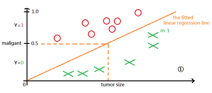
We are given m records of tumor history and come out the fitted linear regression line in grapg labeled ➀, where m-1 th record is identified as non-maligant($Y=0$).

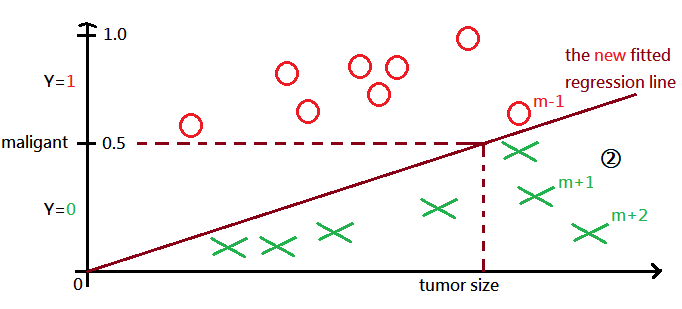
After record m+1, m+2 have been added to the given sample, we get the new fitted regression line in graph labeled ➁, watch out that m-1 th record is now identified as maligant($Y=1$)!!!

Caution must be made that by tradition, the fitted linear regression line could be biased with the input sample and $h_\theta(x)>1\;or\;<\;0$ could happen.

What we want for binary classification in this example is to classify
\(\left\{\begin{array}{l}Y=1,\;h_\theta(x)\geq0.5\\Y=0,\;h_\theta(x)<0.5\end{array}\right.\) The linear regression model is likely to have $h_\theta(x)>1\;or\;<\;0$; while the logistic regression model has $0\leq h_\theta(x)\leq1$!!!

The Logistic Regression Function

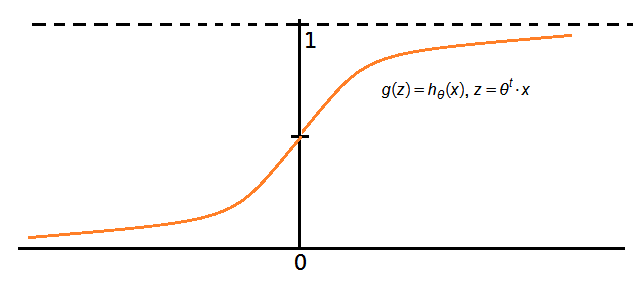
It is also named as the sigmoid function, and defined as: \(h_\theta(x)=\frac1{1+e^{-\theta^t\cdot x}},\;where\;\left\{\begin{array}{l}\theta\in R^n,\;M_{n\times1}\\x\in R^n,\;M_{n\times1}\end{array}\right.\)

We can then have $h_\theta(x)=P(Y=1\vert x;\theta),\;the\;probablity\;of\;Y=1\;given\;x\;and\;\theta$
➀$P(Y=1\vert x;\theta)+P(Y=0\vert x;\theta)=1$
➁$P(Y=1\vert x;\theta)=1-P(Y=0\vert x;\theta)$

The Logistic Regression Cost Function

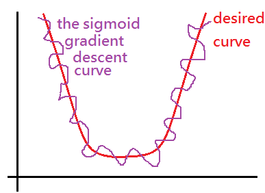
Can we re-using the cost function in linear regression model, $J(\theta)=\frac1{2m}\sum_{i=1}^m(h_\theta(x^{(i)})-y^{(i)})^2$ to be the logistic version of cost function? The answer is no!!! Because the gradient descendent wouldn’t be a smooth convex curve.

The major purpose of the cost function is to reduce the error of the model and gradient descendent could then be applied on to get the $\theta$ that can really have the smallest error.
Two key points must be clarified:
➀when $P(Y=1)\approx1$, the error from 1 for $P(Y=1)\approx0$ ➁when $P(Y=0)\approx0$, the error from 0 for $P(Y=0)\approx0$ We thus define the cost function as:
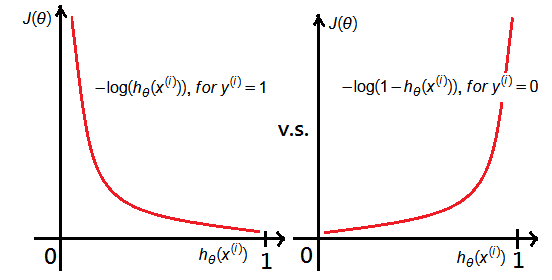
\(\left\{\begin{array}{l}-\log(h_\theta(x)),\;for\;Y=1\\-\log(1-h_\theta(x)),\;for\;Y=0\end{array}\right.\)

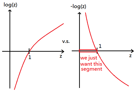
Why do we use log? Why to have a minus sign?

Please recall $\log1=0$, whenever $h_\theta(x)\approx1$ or $h_\theta(x)\approx0$.

Next to formulize it,
\(\begin{array}{l}J(\theta)=\frac1m\sum_{i=1}^m\cos t(h_\theta(x^{(i)}),y^{(i)}),\\where\;\cos t(h_\theta(x^{(i)}),y^{(i)})=\left\{\begin{array}{l}-\log(h_\theta(x^{(i)})),\;for\;y^{(i)}=1\\-\log(1-h_\theta(x^{(i)})),\;for\;y^{(i)}=0\end{array}\right.\end{array}\)

The graph exhibits some findings:
\(\left\{\begin{array}{l}\cos t(h_\theta(x^{(i)}),y^{(i)})=0,\;if\;h_\theta(x^{(i)})=y^{(i)}\\\cos t(h_\theta(x^{(i)}),y^{(i)})\approx\infty,\;if\;h_\theta(x^{(i)})\approx0,\;y^{(i)}=1\\\cos t(h_\theta(x^{(i)}),y^{(i)})\approx\infty,\;if\;h_\theta(x^{(i)})\approx1,\;y^{(i)}=0\end{array}\right.\)

Now, we combine the two cases into one formula:
\(\begin{array}{l}J(\theta)=-\frac1m\sum_{i=1}^m\lbrack y^{(i)}\cdot\log(h_\theta(x^{(i)}))+(1-y^{(i)})\cdot\log(1-h_\theta(x^{(i)}))\rbrack,\\where\;\left\{\begin{array}{l}y^{(i)}=1,\;we\;have\;1-y^{(i)}=0\\y^{(i)}=0,\;we\;have\;1-y^{(i)}=1\end{array}\right.\end{array}\) Thus, we chould have the 2 cases being operated in mutual exclusive flow.

Regularization of The Logistic Regression Cost Function

Please remind the need of regularization of cost function, or you might struggle in the overfitting embarrassed situation. We put an extra term at the end of existing cost function:
\(\begin{array}{l}\underset{REG}{J(\theta)}=-\frac1m\sum_{i=1}^m\lbrack y^{(i)}\cdot\log(h_\theta(x^{(i)}))+(1-y^{(i)})\cdot\log(1-h_\theta(x^{(i)}))\rbrack+\frac\lambda{2m}\sum_{j=1}^n\theta_j^2;\\where\;\theta\in R^n,\;M_{n\times1}\end{array}\)

For the ease of understand, we illustrate by intuition:
➀$\frac{\partial J(\theta)}{\partial\theta_j}=\frac1m\sum_{i=1}^m(h_\theta(x^{(i)})-y^{(i)})\cdot x_j^{(i)},for\;j=1,$ the bias term, no need for regularization!!!
➁$\frac{\partial J(\theta)}{\partial\theta_j}=\frac1m\sum_{i=1}^m(h_\theta(x^{(i)})-y^{(i)})\cdot x_j^{(i)}+\frac\lambda m\theta_j,\;for\;j>1$
;where the term $h_\theta(x^{(i)})-y^{(i)}$ is just the intuitive concept, the proof should make the derivation on the regularized version of cost function, next, we take the action.

Derivate the first part of cost function, we have below deduction:
\(\begin{array}{l}J(\theta)=-\frac1m\sum_{i=1}^m\lbrack y^{(i)}\cdot\log(h_\theta(x^{(i)}))+(1-y^{(i)})\cdot\log(1-h_\theta(x^{(i)}))\rbrack;\\where\;\;h_\theta(x)=\frac1{1+e^{-\theta^t\cdot x}},\;\theta\in R^n,\;x\in R^n,\\\frac{\partial J(\theta)}{\partial\theta_j}=\frac1m\sum_{i=1}^m\lbrack-y^{(i)}\cdot(h_\theta(x^{(i)}))^{-1}-(1-y^{(i)})\cdot(1-h_\theta(x^{(i)}))^{-1}\cdot\frac{\partial{(1-h_\theta(x^{(i)}))}}{\partial\theta_j}\rbrack\end{array}\)

We make further expression:
➀the first order partial differential of $h_\theta(x^{(i)})$:
\(\begin{array}{l}\frac{\partial(h_\theta(x^{(i)}))}{\partial\theta_j}\\=\frac{\partial({\displaystyle\frac1{1+e^{-\theta^t\cdot x^{(i)}}}})}{\partial\theta_j}\\=\frac{\partial(1+e^{-\theta^t\cdot x^{(i)}})^{-1}}{\partial\theta_j}\\=(-1)\cdot\lbrack1+e^{-\theta^t\cdot x^{(i)}}\rbrack^{-2}\cdot(-x_j^{(i)}\cdot e^{-\theta^t\cdot x^{(i)}})\\=\lbrack1+e^{-\theta^t\cdot x^{(i)}}\rbrack^{-2}\cdot(x_j^{(i)}\cdot e^{-\theta^t\cdot x^{(i)}})\end{array}\)

➁extend $1-h_\theta(x^{(i)})$ as:
\(1-h_\theta(x^{(i)})=1-\frac1{1+e^{-\theta^t\cdot x^{(i)}}}=\frac{e^{-\theta^t\cdot x^{(i)}}}{1+e^{-\theta^t\cdot x^{(i)}}}\)

Take ➀ and ➁ into the first order partial differential of $J(\theta)$:
\(\begin{array}{l}\frac{\partial J(\theta)}{\partial\theta_j}\\=\frac1m\sum_{i=1}^m\lbrack-y^{(i)}\cdot(1+e^{-\theta^t\cdot x^{(i)}})\cdot(1+e^{-\theta^t\cdot x^{(i)}})^{-2}\cdot(x_j^{(i)}\cdot e^{-\theta^t\cdot x^{(i)}})+\\(1-y^{(i)})\cdot(\frac{1+e^{-\theta^t\cdot x^{(i)}}}{e^{-\theta^t\cdot x^{(i)}}})\cdot(1+e^{-\theta^t\cdot x^{(i)}})^{-2}\cdot(x_j^{(i)}\cdot e^{-\theta^t\cdot x^{(i)}})\rbrack\\=\frac1m\sum_{i=1}^m\lbrack-y^{(i)}\cdot(1+e^{-\theta^t\cdot x^{(i)}})^{-1}\cdot(x_j^{(i)}\cdot e^{-\theta^t\cdot x^{(i)}})+\\(1-y^{(i)})\cdot e^{\theta^t\cdot x^{(i)}}\cdot(1+e^{-\theta^t\cdot x^{(i)}})^{-1}\cdot(x_j^{(i)}\cdot e^{-\theta^t\cdot x^{(i)}})\rbrack\\=\frac1m\sum_{i=1}^m\lbrack-y^{(i)}\cdot(1+e^{-\theta^t\cdot x^{(i)}})^{-1}\cdot(e^{-\theta^t\cdot x^{(i)}}\cdot x_j^{(i)})+\\(1-y^{(i)})\cdot(1+e^{-\theta^t\cdot x^{(i)}})^{-1}\cdot x_j^{(i)})\rbrack\\=\frac1m\sum_{i=1}^m\lbrack-y^{(i)}\cdot(e^{-\theta^t\cdot x^{(i)}}\cdot x_j^{(i)})+(1-y^{(i)})\cdot x_j^{(i)})\rbrack\cdot(1+e^{-\theta^t\cdot x^{(i)}})^{-1}\\=\frac1m\sum_{i=1}^m\lbrack-y^{(i)}\cdot(e^{-\theta^t\cdot x^{(i)}}\cdot x_j^{(i)})+(1-y^{(i)})\cdot x_j^{(i)})\rbrack\cdot h_\theta(x^{(i)})\end{array}\)

Finally, take the second part together in the derivative, we get the total solution:
\(\frac{\partial J(\theta)_{REG}}{\partial\theta}=\frac{\displaystyle1}{\displaystyle m}\sum_{i=1}^m\lbrack-x^{(i)}\cdot y^{(i)}\cdot e^{-\theta^t\cdot x^{(i)}}+x^{(i)}\cdot(1-y^{(i)})\rbrack\cdot h_\theta(x^{(i)})+\frac\lambda m\theta\)

Multiple Classification

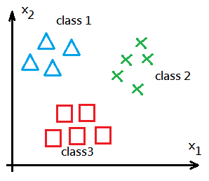
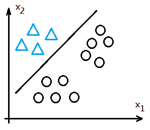
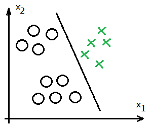
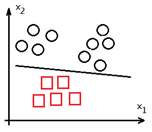
We now migrate to multiple classification. There might exist more than one pattern in the given sampling, how do you plan to classify the object to the correct identity? We introduce the most often used method, one-versus-all.
Take $h_\theta^{(k)}(x^{(i)})=P(y^{(i)}=k\vert\theta^{(k)},x^{(i)});\;k=1,2,3,\;i=1\;to\;m,\;the\;count\;of\;data\;set$. Next to illustrate one-versus-all method:

➀train with $h_\theta^{(1)}(x^{(i)})$ to get the desired $\theta^{(1)}$ vector for class 1.

➁train with $h_\theta^{(2)}(x^{(i)})$ to get the desired $\theta^{(2)}$ vector for class 2.

➂train with $h_\theta^{(3)}(x^{(i)})$ to get the desired $\theta^{(3)}$ vector for class 3.

After $\theta^{(k)}$ has been figured out, for any new input of $x^{(i)}$, where $i\geq m$, use $h_\theta^{(k)}(x^{(i)})$ to predict the output, and choose the maximum one as the object identity.

That is to say $\underset k{max}\;h_\theta^{(k)}(x^{(i)})$ as the identity of class k.

Overfitting versus Regularization

11 Nov 2017

Regularization

Regularization aims at overfitting elimination; whereas underfitting should be improived by adding extra features in your hypothesis model.

Overfitting

Overfitting usually occurs with the symptom that the hypothesis model fits very well to the training data, but, when the model is processing the real thing, it wouldn’t predict as well as it had estimated in training stage.

Regularization by means of Lagrangian

When we suspect our hypothesis model is overfitting, it should have been regularized by means of lagrange multiplier. For the ease of explain and better understand, in this article, we’d like to illustrate with linear regression model.
Take the cost function $J(\theta)=\frac1{2m}\sum_{i=1}^m(h_\theta(x^{(i)})-y^{(i)})^2$, where the purpose of S.L.R is to minimize $J(\theta)$. Suppose that you already realize what cost function is for.
Given $h_\theta(x)=\theta^t\cdot x$, where \(\theta=\begin{bmatrix}\theta_1\\\theta_2\end{bmatrix}\) is the coefficients.
Take \(X=\begin{bmatrix}x_1\\x_2\end{bmatrix}\) as the input data, and $x_1=1$, it is the intercept, or the bias term. The superscribe(i) of $X$, $Y$ are the index of the input data record, means it is the i-th input data $X$, $Y$.
Now, put an extra item after the cost function could we regularize our existsing cost function:
\(\begin{array}{l}\underset\theta{min}\;J(\theta)=\frac1{2m}(\sum_{i=1}^m(h_\theta(x^{(i)})-y^{(i)})^2+\lambda\sum_{j=1}^n\theta_j^2);\;where\;h_\theta(x)=\theta^t\cdot x\\\theta_j=\theta_j-\;\frac\alpha m\frac{\partial J(\theta)}{\partial\theta_j}\\\;\;\;\;=\theta_j-\frac\alpha m\sum_{i=1}^m(h_\theta(x^{(i)})-y^{(i)})\cdot x_j^{(i)}-\frac\lambda m\theta_j;\;for\;j=1\;to\;n\end{array}\)

Why Lagrangian Achieves Regularization?

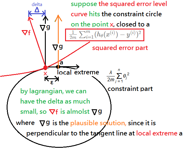
Suppose you all realize and have the basic intuition about lagrange multiplier. In this section, we will take the squared error part as the level curve, and is it subject to the constraint function of circle.
Suppose again, the level curve hits the circle on the point $x$, very very close to the local extreme point of the circle, say it $a$. We’d like to bring down the delta($\delta$) as much as closed to zero, that is $\nabla f\approx\nabla g$.
Since the $\nabla g$ if the normal vector and is perpendicular to the local extreme point $a$, then, we can then believe that we have reduced the projection error of delta($\delta$), $\nabla f$ would be as plausible solution as $\nabla g$.

In the next topic, we will further illustrate regularization in logistic regression for binary classification.

Gradient Descendent

07 Nov 2017

Gradient Descendent

Most widely used in machine learning with respect to linear regression, logistic regression for supervised learning. But, the gradient descendent itself actually knows nothing when to stop!!

Begin from Cost Function in Simple Linear Regressoin(S.L.R)

take the cost function $J(\theta)=\frac1{2m}\sum_{i=1}^m(h_\theta(x^{(i)})-y^{(i)})^2$, where the purpose of S.L.R is to minimize $J(\theta)$.
given $h_\theta(x)=\theta^t\cdot x$, where \(\theta=\begin{bmatrix}\theta_1\\\theta_2\end{bmatrix}\) is the coefficients
take \(X=\begin{bmatrix}x_1\\x_2\end{bmatrix}\) as the input data
and $x_1=1$, it is the intercept, or the bias term.
as to the divide by 2m is an artificial design:
➀$\frac12$ is to eliminate the power of 2 in the square, after differentiation is taken.
➁$\frac1m$ is to average all squared errors of m input rows of data.
➂the superscribe(i) of $X$, $Y$ are the index of the input data record, means it is the i-th input data $X$, $Y$

Step into Gradient ∇ of $J(\theta)$

suppose we are given m records of input data, they are $X$ and $Y$. ➀take derivation of $J\left(\theta \right)$ on ${\theta }_j$, then we obtain:

$\frac{\partial J\left(\theta \right)}{\partial {\theta }_j}=\frac{1}{m}\sum _{i=1}^m\left(h_{\theta }\right(x^{\left(i\right)})-y^{\left(i\right)})·x_j^{\left(i\right)}$

since we are running batch gradient descendent, $\frac{1}{m}$ is required to average it.
➁if m = 1, then, we just have the j-th term as:

$\frac{\partial J\left(\theta \right)}{\partial {\theta }_j}=\sum _{i=1}^m\left(h_{\theta }\right(x^{\left(i\right)})-y^{\left(i\right)})·x_j^{\left(i\right)}$

Learning Rate α

it is used to converge the result of gradient descendent. The smaller value would believed to have a less fluctuation.

Put It Together

put everything together, we will have the j-the term of $\theta$, it is inclusive of the bias term $\theta_1$:

${\theta }_j={\theta }_j-\alpha ·\frac{1}{m}\sum _{i=1}^m\left(h_{\theta }\right(x^{\left(i\right)})-y^{\left(i\right)})·x_j^{\left(i\right)}, where j=1 to n, \theta \in R^n$

given $X\in M_{m\times n}, \theta \in M_{n\times 1}, Y\in M_{m\times 1}, x^{\left(i\right)}\in M_{n\times 1}$,

$X={\left[\begin{array}{c}-(x^{\left(1\right)}{)}^t-\\ -(x^{\left(2\right)}{)}^t-\\ ...\\ -(x^{\left(m\right)}{)}^t-\end{array}\right]}_{mxn}$

and, we just deduce out:

$$\begin{gathered} \frac{\partial J\left(\theta \right)}{\partial {\theta }_j}=\frac{1}{m}\sum _{i=1}^m\left(h_{\theta }\right(x^{\left(i\right)})-y^{\left(i\right)})·x_j^{\left(i\right)} \\ =({\left[\begin{array}{c}-(x^{\left(1\right)}{)}^t-\\ -(x^{\left(2\right)}{)}^t-\\ ...\\ -(x^{\left(m\right)}{)}^t-\end{array}\right]}_{mxn}·{\left[\begin{array}{c}{\theta }_1\\ {\theta }_2\\ ...\\ {\theta }_n\end{array}\right]}_{n\times 1}-{\left[\begin{array}{c}{y}^{\left(1\right)}\\ y^{\left(2\right)}\\ ...\\ y^{\left(m\right)}\end{array}\right]}_{m\times 1}{)}^t·\left[\begin{array}{c}{x}_j^{\left(1\right)}\\ x_j^{\left(2\right)}\\ ...\\ x_j^{\left(m\right)}\end{array}\right]·\frac{1}{m} \end{gathered}$$

Why the Gradient Descendent Works?

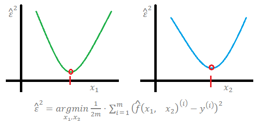
We will illustrate with cost function of multiple parameters:

➀given $f(x_1,x_2)$ a multi-parameters cost function, the gradient ∇ of $f$ are $\frac{\partial f}{\partial x_1}$, $\frac{{\displaystyle \partial f}}{{\displaystyle \partial x_2}}$
➁suppose $y=f(x_1,x_2)$
➂take ${\hat{\epsilon }}^2=\frac{1}{2m}·\sum _{i=1}^m\left(\hat{f}\right(x_1,x_2{)}^{\left(i\right)}-y^{\left(i\right)}{)}^2$
➃to get the minimum value of ${\hat{\epsilon }}^2$, we have to figure out by below function:

${\hat{\epsilon }}^2=\underset{x_1,x_2}{argmin}\frac{1}{2m}·\sum _{i=1}^m\left(\hat{f}\right(x_1,x_2{)}^{\left(i\right)}-y^{\left(i\right)}{)}^2$

, where ${\hat{\epsilon }}^2$ is a convex function
➄the gradient descendent is the algorithm that can gradually lead to final $x_1$, $x_2$ that can minimize ${\hat{\epsilon }}^2$

suppose we are beginning from some base point ${x_1}^{\left(0\right)}$, ${x_2}^{\left(0\right)}$, where the upper subscribe(0) is the iteration index, indicates that it is the 0-th iteration.

for $i$=0 to some large value.
➀${x_1}^{\left(i\right)}={x_1}^{(i-1)}-\alpha ·\frac{\partial f({x_1}^{(i-1)}, {x_2}^{(i-1)})}{\partial x_1}$
➁${x_2}^{\left(i\right)}={x_2}^{(i-1)}-\alpha ·\frac{\partial f({x_1}^{(i-1)}, {x_2}^{(i-1)})}{\partial x_2}$
repeat above 2 steps in the same iteration, loop until the ${\hat{\epsilon }}^2$ could be believed at its minimum or the iteration index i is large enough.

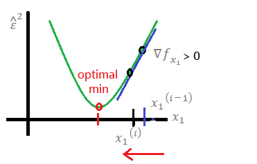
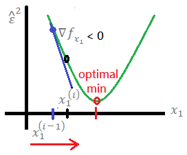
next, we explain why we choose to minimize the gradient, actually, there exists 2 gradients, +∇ and −∇:
➀for +∇, the equation minus the positive gradient at learning rate α > 0, then, ${x_1}^{\left(i\right)}={x_1}^{(i-1)}-\alpha ·\nabla f_{x_1}({x_1}^{(i-1)},{x_2}^{(i-1)})$
the ${x_1}^{\left(i\right)}$ would step back to the optimal minimum.

➁for −∇, the equation minus the negative gradient at learning rate α > 0, then, ${x_1}^{\left(i\right)}={x_1}^{(i-1)}+\alpha ·\nabla f_{x_1}({x_1}^{(i-1)},{x_2}^{(i-1)})$
the ${x_1}^{\left(i\right)}$ would step forward to the optimal minimum.

both ➀, ➁ work for $x_2$ in this example, we thus prove it!!

QR Decomposition

31 Oct 2017

QR Decomposition

QR decomposition claims that A = B⋅X = B⋅D⋅E⋅X = Q⋅R. This article will show you the way to prove it, we will begin from Gram-Schmit Procedure, then, briefly introduce to the projection matrix, then, migrate to triangular matrix, finally to prove the QR decomposition.

Gram-Schmit Procedure

Given a set of linear independent vectors set S = {v₁, v₂,…, v_p} ∈ R^m,
define vectors u_i, 1 ≤ i ≤ p by
u_i = v_i − [((v_i)^t ⋅ u₁) ∕ ((u₁)^t ⋅ u₁)] ⋅ u₁ − [((v_i)^t ⋅ u₂) ∕ ((u₂)^t ⋅ u₂)] ⋅ u₂ − [((v_i)^t ⋅ u₃) ∕ ((u₃)^t ⋅ u₃)] ⋅ u₃ − … − [((v_i)^t ⋅ u_i−1) ∕ ((u_i−1)^t ⋅ u_i−1)] ⋅ u_i−1
the set T = {u₁, u₂,…, u_p} is a linear independent orthonormal set and aoan(S) = span(T)
we just have below holds:
u₁ = v₁
u₂ = v₂ − [((v₂)^t ⋅ u₁) ∕ ((u₁)^t ⋅ u₁)] ⋅ u₁
u₃ = v₃ − [((v₃)^t ⋅ u₁) ∕ ((u₁)^t ⋅ u₁)] ⋅ u₁ − [((v₃)^t ⋅ u₂) ∕ ((u₂)^t ⋅ u₂)] ⋅ u₂
u₄ = v₄ − [((v₄)^t ⋅ u₁) ∕ ((u₁)^t ⋅ u₁)] ⋅ u₁ − [((v₄)^t ⋅ u₂) ∕ ((u₂)^t ⋅ u₂)] ⋅ u₂ − [((v₄)^t ⋅ u₃) ∕ ((u₃)^t ⋅ u₃)] ⋅ u₃
…
u_p = v_p − [((v_p)^t ⋅ u₁) ∕ ((u₁)^t ⋅ u₁)] ⋅ u₁ − [((v_p)^t ⋅ u₂) ∕ ((u₂)^t ⋅ u₂)] ⋅ u₂ − … − [((v_p)^t ⋅ u_p−1) ∕ ((u_p−1)^t ⋅ u_p−1)] ⋅ u_p−1

Prove Gram-Schmit Procedure by means of Projection Matrix

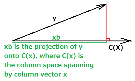
Begin by projection matrix to prove Gram-Schmit Procedure illustrated in below pic:

take x ⋅ b = y_proj, the projection of y onto C(x), where C(x) is the column space spanned by vector x
C(x) ⊥ (y − x ⋅ b), then
=>C(x) ⋅ (y − x ⋅ b) = 0,
=>x^t ⋅ (y − x ⋅ b) = 0,
=>x^t ⋅ x ⋅ b = x^t ⋅ y,
=>b = (x^t ⋅ x)⁻ ⋅ x^t ⋅ y; where (x^t ⋅ x)⁻ is the generalized inverse form,
=>y_proj = x ⋅ (x^t ⋅ x)⁻ ⋅ x^t ⋅ y
∵x is itself a column vector, then (x^t ⋅ x)⁻ = (x^t ⋅ x)⁻¹ just holds, for the vector x is in the spanning set/basis
∴y_proj = [(x^t ⋅ y) ∕ (x^t ⋅ x)] ⋅ x = [(y^t ⋅ x) ∕ (x^t ⋅ x)] ⋅ x

To further explain Gram-Schmit Procedure in terms of Projection Matrix:

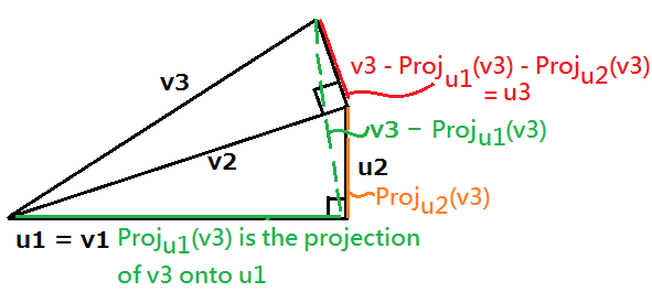
take y as v₂, x as u₁, where u₁ = v₁, then
u₂ = v₂ − [((u₁)^t ⋅ v₂) ∕ ((u₁)^t ⋅ u₁)] ⋅ u₁, where the second term is just the projection of v₂ onto u₁
u₃ = v₃ − Proj_w2(v₃), where w₂ = Span(u₁, u₂)
     = v₃ − Proj_u1(v₃) − Proj_u2(v₃)
     = v₃ − [((u₁)^t ⋅ v₃) ∕ ((u₁)^t ⋅ u₁)] ⋅ u₁ − [((u₂)^t ⋅ v₃) ∕ ((u₂)^t ⋅ u₂)] ⋅ u₂
the flow is exhibited by below pic:

u₄ = v₄ − Proj_w3(v₄), where w₃ = Span(u₁, u₂, u₃)
     = v₄ − [((u₁)^t ⋅ v₄) ∕ ((u₁)^t ⋅ u₁)] ⋅ u₁ − [((u₂)^t ⋅ v₄) ∕ ((u₂)^t ⋅ u₂)] ⋅ u₂ − [((u₃)^t ⋅ v₄) ∕ ((u₃)^t ⋅ u₃)] ⋅ u₃
…
finally, we can reach
u_p = v_p − [((u₁)^t ⋅ v_p) ∕ ((u₁)^t ⋅ u₁)] ⋅ u₁ − [((u₂)^t ⋅ v_p) ∕ ((u₂)^t ⋅ u₂)] ⋅ u₂ − … − [((u_p−1)^t ⋅ v_p) ∕ ((u_p−1)^t ⋅ u_p−1)] ⋅ u_p−1

Further refine the notation in Gram-Schmit and Formula Representation:

take S = {v₁, v₂,…, v_p} to be S = {a₁, a₂,…, a_p}
take T = {u₁, u₂,…, u_p} to be T = {b₁, b₂,…, b_p}
b₁ = a₁
b₂ = a₂ − [((b₁)^t ⋅ a₂) ∕ ((b₁)^t ⋅ b₁)] ⋅ b₁
b₃ = a₃ − [((b₁)^t ⋅ a₃) ∕ ((b₁)^t ⋅ b₁)] ⋅ b₁ − [((b₂)^t ⋅ a₃) ∕ ((b₂)^t ⋅ b₂)] ⋅ b₂
b₄ = a₄ − [((b₁)^t ⋅ a₄) ∕ ((b₁)^t ⋅ b₁)] ⋅ b₁ − [((b₂)^t ⋅ a₄) ∕ ((b₂)^t ⋅ b₂)] ⋅ b₂ − [((b₃)^t ⋅ a₄) ∕ ((b₃)^t ⋅ b₃)] ⋅ b₃
…
b_p = a_p − [((b₁)^t ⋅ a_p) ∕ ((b₁)^t ⋅ b₁)] ⋅ b₁ − [((b₂)^t ⋅ a_p) ∕ ((b₂)^t ⋅ b₂)] ⋅ b₂ − [((b₃)^t ⋅ a_p) ∕ ((b₃)^t ⋅ b₃)] ⋅ b₃ − … − [((b_p−1)^t ⋅ a_p) ∕ ((b_p−1)^t ⋅ b_p−1)] ⋅ b_p−1
At this moment, the proof has validated Gram-Schmit by the projection matrix

Express Gram-Schmit Procedure in Matrix Product

Advance one step to represent Gram-Schmit Procedure by matrix product:

if we take X_i,j = ((b_i)^t ⋅ a_j) ∕ ((b_i)^t ⋅ b_i), then, we could have:
b₁ = a₁
b₂ = a₂ − X_1,2 ⋅ b₁
b₃ = a₃ − X_1,3 ⋅ b₁ − X_2,3 ⋅ b₂
b₄ = a₄ − X_1,4 ⋅ b₁ − X_2,4 ⋅ b₂ − X_3,4 ⋅ b₃
…
b_p = a_p − X_1,p ⋅ b₁ − X_2,p ⋅ b₂ − X_3,p ⋅ b₃ − … − X_p−2,p ⋅ b_p−2 − X_p−1,p ⋅ b_p−1

Then, express a_i in terms of b_i′s:

a₁ = b₁
a₂ = b₂ + X_1,2 ⋅ b₁
a₃ = b₃ + X_1,3 ⋅ b₁ + X_2,3 ⋅ b₂
a₄ = b₄ + X_1,4 ⋅ b₁ + X_2,4 ⋅ b₂ + X_3,4 ⋅ b₃
…
a_p = b_p + X_1,p ⋅ b₁ + X_2,p ⋅ b₂ + X_3,p ⋅ b₃ + … + X_p−2,p ⋅ b_p−2 + X_p−1,p ⋅ b_p−1

Further refine:

take X_i,i = 1, that is
a₁ = X_1,1 ⋅ b₁
a₂ = X_1,2 ⋅ b₁ + X_2,2 ⋅ b₂
a₃ = X_1,3 ⋅ b₁ + X_2,3 ⋅ b₂ + X_3,3 ⋅ b₃
a₄ = X_1,4 ⋅ b₁ + X_2,4 ⋅ b₂ + X_3,4 ⋅ b₃ + X_4,4 ⋅ b₄
…
a_p = X_1,p ⋅ b₁ + X_2,p ⋅ b₂ + X_3,p ⋅ b₃ + … + X_p−2,p ⋅ b_p−2 + X_p−1,p ⋅ b_p−1 + X_p,p ⋅ b_p

take X as an upper unit triangular matrix where Xi,i = 1 
X = 
X1,1 X1,2 X1,3 X1,4 .... X1,p  
 0    X2,2 X2,3 X2,4 .... X2,p
 0     0   X3,3 X3,4 .... X3,p
 0     0    0   X4,4 .... X4,p
   ..................
 0     0    0   0  ....   Xp,p

then,
A_m×p = [a₁|a₂|…|a_p], where a_i ∈ R^m,
B_m×p = [b₁|b₂|…|b_p], where b_i ∈ R^m,

take D = diag(||b₁||⁻¹, ||b₂||⁻¹, ||b₃||⁻¹,…,||b_p||⁻¹)
take Q = B ⋅ D = diag(b₁ ∕ ||b₁||, b₂ ∕ ||b₂||, b₃ ∕ ||b₃||,…, b_p ∕ ||b_p||)
take E = diag(||b₁||, ||b₂||, ||b₃||,…,||b_p||)…to eliminate D
take R = E ⋅ X = [(||b₁|| ⋅ X₁)|(||b₂|| ⋅ X₂)|(||b₃|| ⋅ X₃)|,…,|(||b_p|| ⋅ X_p)]…upper triangular matrix
then, A = B ⋅ X = B ⋅ D ⋅ E ⋅ X = Q ⋅ R …QR decomposition, where such Q ⋅ R is unique, ∵B ⋅ X is also unique, too.