27 Nov 2017
Initial Idea
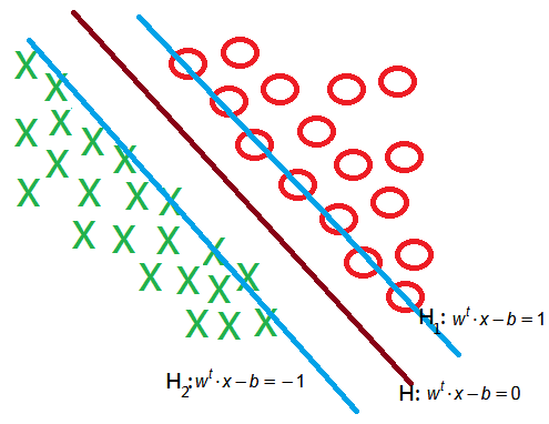
Now, we know the distance from $H$ to $H_1$ is $\frac{\left|w^t\cdot x-b\right|}{\left\|w\right\|}=\frac1{\left\|w\right\|}$; where $H_1:w^t\cdot x-b=1$. As to distance between $H_1$ and $H_2$,
we must minimize the term $\left\|w\right\|=(w^t\cdot w)^{\textstyle\frac12}$ to satisfy the condition that no points between $H_1$ and $H_2$.
More precisely, by minimizing $w^t\cdot w$, we expect to have:
➀for positive examples, $w^t\cdot x-b\geq1$, where $y=1$.
➁for negative examples, $w^t\cdot x-b\leq-1$, where $y=-1$.
Then, combine ➀ and ➁ we can have:
\(y_i\cdot(w^t\cdot x_i-b)\geq1\), \(\forall i\in\{1,2,...,n\}\)
We can formulate our problem as:
$\underset w{min}\frac12w^t\cdot w$, subject to $y_i\cdot(w^t\cdot x_i-b)\geq1,\forall i$.
The first part is the target, the second part is the constraint.
We introduce $\alpha_1,\alpha_2,\dots\alpha_n$ to be the lagrange multiplier and express in below lagrangian to be our objective function:
\(L(w,b,\alpha)=\frac12w^t\cdot w-\sum_{i=1}^n\alpha_i\cdot(y_i\cdot(w^t\cdot x_i-b)-1)\)
;where $L$ is actually the maximum likelihood function for $w$, $\alpha$, $b$ to be estimated out the best optimal value at the corresponding largest possibility.
Regularize The Objective Function
Next to inspect inside $L(w,b,\alpha)$ to get the best optimal value of $w$, $\alpha$, $b$:
\(\begin{array}{l}L(w,b,\alpha)\\=\frac12w^t\cdot w-\sum_{i=1}^n\alpha_i\cdot(y_i\cdot(w^t\cdot x_i-b)-1)\\=\frac12w^t\cdot w-\sum_{i=1}^n\alpha_i\cdot y_i\cdot(w^t\cdot x_i-b)+\sum_{i=1}^n\alpha_i\end{array}\)
To get the optimal $\alpha$, we should take partial derivatives of $L$ on $w$, $b$ respectively and equate them to zero:
➀$\frac{\partial L}{\partial w}=w-\sum_{i=1}^n\alpha_i\cdot y_i\cdot x_i=0$, then, we have $w=\sum_{i=1}^n\alpha_i\cdot y_i\cdot x_i$
➁$\frac{\partial L}{\partial b}=\sum_{i=1}^n\alpha_i\cdot y_i$
➂use the deduction result of ➀ and ➁ in $L(w,b,\alpha)$, we obtain:
\(\begin{array}{l}L(w,b,\alpha)\\=\frac12(\sum_{i=1}^n\alpha_i\cdot y_i\cdot x_i)^t\cdot(\sum_{i=1}^n\alpha_i\cdot y_i\cdot x_i)\\-\sum_{i=1}^n\alpha_i\cdot y_i\cdot((\sum_{i=1}^n\alpha_i\cdot y_i\cdot x_i)^t\cdot x_i-b)\\+\sum_{i=1}^n\alpha_i\end{array}\)
➃reduce from the second term, we have below deduction:
\(\begin{array}{l}\sum_{i=1}^n\alpha_i\cdot y_i\cdot((\sum_{i=1}^n\alpha_i\cdot y_i\cdot x_i)^t\cdot x_i-b)\\=\sum_{i=1}^n\alpha_i\cdot y_i\cdot(\sum_{i=1}^n\alpha_i\cdot y_i\cdot x_i)^t\cdot x_i\\-\sum_{i=1}^n\alpha_i\cdot y_i\cdot b\\=(\sum_{i=1}^n\alpha_i\cdot y_i\cdot x_i)^t\cdot(\sum_{i=1}^n\alpha_i\cdot y_i\cdot x_i)\\\dots\sum_{i=1}^n\alpha_i\cdot y_i\cdot b=0\end{array}\)
➄take it back to $L(w,b,\alpha)$, we get:
\(\begin{array}{l}L(w,b,\alpha)\\=-\frac12(\sum_{i=1}^n\alpha_i\cdot y_i\cdot x_i)^t\cdot(\sum_{i=1}^n\alpha_i\cdot y_i\cdot x_i)\\+\sum_{i=1}^n\alpha_i\\=-\frac12\sum_{i,j=1}^n\alpha_i\cdot\alpha_j\cdot y_i\cdot y_j\cdot(x_i^t\cdot x_j)\\+\sum_{i=1}^n\alpha_i\end{array}\)
Why $L(w,b,\alpha)$ = the target plus the constraint?
But, why do we design $L(w,b,\alpha)$ in the expression of the target plus the constraint? Recall that in the lagrange multiplier article, I have shown you by taking $L(x,\lambda)=f(x)+\lambda\cdot g(x)$, finally leads to $\lambda<0$.
➀if we choose $L(x,\lambda)=f(x)-\lambda\cdot g(x)$, then $\lambda>0$. This is by artificial design. Whether plus or minus sign is used in the expression, could we have the similar achievement.
➁now, back to the formulate of our problem:
$\underset{w,b}{min}\frac12w^t\cdot w$, subject to $y_i\cdot(w^t\cdot x_i-b)\geq1$
➂suppose we take the constraint function function to be $g(x)=y_i\cdot(w^t\cdot x_i-b)\geq1$, if $\lambda$ would be negative by prior lagrangian proof, to get positive $\lambda$, we should use the minus operator in $L(x,\lambda)$.
➃Therefore, almost all SVM articles design $L(w,b,\alpha)$; where $\alpha$ is the lagrange multiplier given in the expression by using the minus operator:
\(L(w,b,\alpha)=\frac12w^t\cdot w-\sum_{i=1}^n\alpha_i\cdot(y_i\cdot(w^t\cdot x_i-b)-1)\)
➄such design guarantees that we could have $\forall\alpha_i>0$, which would be one major condition that must be satisfied in the following SVM article.
After solving the $\alpha_i$, we can get $w=\sum_{i=1}^n\alpha_i\cdot y_i\cdot x_i$, then, we can classify a new object x by:
\(\begin{array}{l}f(x)\\=sign(w^t\cdot x-b)\\=sign((\sum_{i=1}^n\alpha_i\cdot y_i\cdot xi)^t\cdot x-b)\\=sign(\sum_{i=1}^n\alpha_i\cdot y_i\cdot(xi)^t\cdot x-b)\end{array}\)
Non-Linear Training Set
Here, we have a question, what, if the separating surface of the two classes is not linear?
This might imply that the training set is distributed in a non-linear pattern. Suggestion would be made to transform the training set into another high-dimensional(maybe) space, such that they could be linearly separable.
➀let $\Phi(\cdot)$ to be the transformation function to some high-dimensional space, then:
\(\begin{array}{l}L(\alpha)\\=-\frac12\sum_{i,j=1}^n\alpha_i\cdot\alpha_j\cdot y_i\cdot y_j\cdot(\Phi(x_i).\times\Phi(x_j))\\+\sum_{i=1}^n\alpha_i\end{array}\)
, where $k(x_i,x_j)=\Phi(x_i).\times\Phi(x_j)$, $k(x_i,x_j)$ is the kernel function, the element-wise dot product $\Phi^t(x_i).\times\Phi(x_j)$ in the high-dimensional space is equivalent to the kernel function of the space of the output(or maybe input) parameters.
➁we can take $k(x_i,x_j)=e^{-(\frac{\left|x_i-x_j\right|^2}{2\cdot\delta^2})}$,
where, $k(x_i,x_j)\in R^{n2},\Phi(x_i).\times\Phi(x_j)\in R^{n2}$
$x_i,x_j\in R^{n1}$ and $n1\leq n2$.
25 Nov 2017
Prologue To Support Vector Machine
Given training data set of size $n$, where they are {($x_1$, $y_1$), ($x_2$, $y_2$),...,($x_n$, $y_n$)}, $\forall x_i\in R^d$, $\forall y_i\in\{+1,-1\}$.
Supposed these data could be classified and we'd like to learn a hyperplane classifier:
$$f(x)=sign(w^t\cdot x-b)$$
Separating Hyperplane With Minimum Safe Guard
Furthermore, we want this hyperplane to have the minimum separating margin with respect to the two classes.

Specifically, if all goes well, there shall exist no data points in between $H_1$ and $H_2$.
\(\begin{array}{l}H:w^t\cdot x-b=0\\H_1:w^t\cdot x-b=1\\H_2:w^t\cdot x-b=-1\\\\\end{array}\)
For any separaing $H$ and the corresponding $H_1$ and $H_2$, we can solve by normalizing the coefficient vector $w$, such that $H_1$ and $H_2$ exist.
proof:
➀suppose $H_1:a^t\cdot x-b_1=0$ and $H_1:a^t\cdot x-b_2=0$ are two parallel hyperplanes. Since they are parallel, they can have the same weight $a$.
➁take $\overline b=\frac{b_1+b_2}2$ and $\delta=b_1-\overline b=\overline b-b_2$
\(\begin{array}{l}\therefore H_1:a^t\cdot x-(\delta+\overline b)=0\\\;\;\;\;H_2:a^t\cdot x-(\overline b-\delta)=0\\\therefore H_1:a^t\cdot x-\overline b=\delta\\\;\;\;\;H_2:a^t\cdot x-\overline b=-\delta\\\end{array}\)
➂then, divide both equality by $\delta$, we obtain:
\(\begin{array}{l}H_1:\frac{a^t}\delta\cdot x-\frac{\overline b}\delta=1\\H_2:\frac{a^t}\delta\cdot x-\frac{\overline b}\delta=-1\\\\\end{array}\)
➃take $w=\frac{a^t}\delta$ and $b=\frac{\overline b}\delta$, could we get our expected $H_1$ and $H_2$.
Next would be to maximize the distance between $H_1$ and $H_2$, therefore, there will be some positive examples on $H_1$, some negative examples on $H_2$.
These examples are called support vectors, only they participate in the separating hyperplane $H_1$ and $H_2$, other examples could be removed or moved around, since they didn’t cross $H_1$, $H_2$.
Distance Measurement Of Point To Line
Before step into support vector machine, have a galance at the measurement of distance from point to line.

By given $a\cdot x+b\cdot y+c=0$ is a line parametric equation, then, $\frac ab\cdot x+y+\frac cb=0$; therefore, $y=-\frac ab\cdot x-\frac cb$ has slope $-\frac ab$.
➀pointers on this line could be expressed as below:
\(\begin{bmatrix}x\\-\frac ab\cdot x-\frac cb\end{bmatrix}=\begin{bmatrix}0\\-\frac cb\end{bmatrix}+(-\frac1b)\cdot\begin{bmatrix}-b\\a\end{bmatrix}\cdot x\)
➁therefore, \(\begin{bmatrix}-b\\a\end{bmatrix}\) is the vector parallel to this line, and \(\begin{bmatrix}a\\b\end{bmatrix}\) is the vector perpendicular to the line.
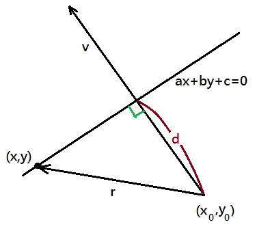
➂take $r=(x-x_0,y-y_0)$, by projecting $r$ onto $v$, then, we can deduce out $\left|Proj_v\cdot r\right|=\frac{\left|v^t\cdot r\right|}{\left|v\right|}$ to be the distance.
Since $v^t\cdot(r-v\cdot k)=0$, therefore, $k=\frac{v^t\cdot r}{v^t\cdot v}$,
\(\begin{array}{l}d=\left\|v\cdot\frac{v^t\cdot r}{v^t\cdot v}\right\|\\=\left\|\frac v{v^t\cdot v}\cdot v^t\cdot r\right\|\\=\left\|v\cdot(v^t\cdot v)^{-1}\cdot v^t\cdot r\right\|\\=\left\|(v^t)^{-1}\cdot v^t\cdot r\right\|\\=\frac{\left\|v^t\cdot r\right\|}{\left\|v^t\right\|}=\frac{\left\|v^t\cdot r\right\|}{\left\|v\right\|}\end{array}\)
➃suppose ($x$,$y$) is on $H$, by taking the absolute value of projecting $r$ onto $v$, we can get the distance from $H$ to $H_1$:
\(\begin{array}{l}\left|Proj_v\cdot r\right|\\=\frac{\left\|v^t\cdot r\right\|}{\left\|v\right\|},v=\left\langle a,b\right\rangle\\=\frac{\left|a\cdot(x-x_0)+b\cdot(y-y_0)\right|}{\sqrt{a^2+b^2}}\\=\frac{\left|a\cdot x+b\cdot y-(a\cdot x_0+b\cdot y_0)\right|}{\sqrt{a^2+b^2}}\\=\frac{\left|0-(-c)\right|}{\sqrt{a^2+b^2}}\\=\frac c{\sqrt{a^2+b^2}}\\=\frac{\left|a\cdot x_0+b\cdot y_0\right|}{\sqrt{a^2+b^2}}\end{array}\)
20 Nov 2017
Neural Network Backward Propagation
Backward propagation is for the deduction of the $\theta_{i,j}^{(\mathcal l)}$ that could bring the error in the cost function to a minimum state. In neural network, gradient descendent
is a mandatory mean to reach the $\theta_{i,j}^{(\mathcal l)}$ to the local minimum, and together with regularization to have an optimal approximation. Backward propagation proceeds in the reversed order
and propagate the error from the final last one layer back to the the final last two layer, until the second layer, the algorithm would facilitate the whole gradient descendent process to find its local minimum.
The Regularized Neural Network Cost Function
The complete regularized cost function consists of two parts, part one is the cost function itself, part two is the regularized term:
\(\begin{array}{l}\underset{REG}{J(\theta)}=\frac1m\sum_{i=1}^m\sum_{k=1}^K\left[-y_k^{(i)}\cdot\log(h_\theta^{(k)}(x^{(i)}))-(1-y_k^{(i)})\cdot\log(1-h_\theta^{(k)}(x^{(i)}))\right]\\+\frac\lambda{2m}\sum_{\mathcal l=1}^{L-1}\sum_{j=1}^{j_\mathcal l}\sum_{k=1}^{k_\mathcal l}(\theta_{j,k}^{(\mathcal l)})^2\\,where\;h_\theta(x)\in R^K\\\end{array}\)
Suppose we are given totally m input data, the model where the cost function belongs to comes out with K outputs, and you all know that gradient descendent would be proceeded with derivation of $J(\theta)$ taken on the ($i,j$)th term in the weighting matrix $\theta^{(\mathcal l)}$ in between layer $\mathcal l$ and $\mathcal l+1$.
To make it more clear for the proof in next section, whenever you read $\theta_{i,j}^{(\mathcal l)}$, in this article, they are:
➀the weighting matrix $\theta^{(\mathcal l)}$ in between layer $\mathcal l$ and $\mathcal l+1$.
➁$i$ is the $i$-th row of the weighting matrix $\theta^{(\mathcal l)}$, it is also the $i$-th activation function in next layer $\mathcal l+1$.
➂{j} is the $j$-th output from the activation function at layer $\mathcal l$.
➃$\theta_{i,j}^{(\mathcal l)}$ translates the $j$-th output from the activation function at layer $\mathcal l$ into one of the input of the $i$-th activation function in next layer $\mathcal l+1$!!!!
All we need to compute are $J(\theta)$ and $\frac{\partial J(\theta)}{\partial\theta_{i,j}^{(\mathcal l)}}$ in a gradient descendent manner, the point is how to achieve the goal and why!
The Gradient Computation By Intuition
Take the cost function by intuition:
\(J(\theta)=-y^{(i\_data)}\cdot\log(h_\theta(x^{(i\_data)}))-(1-y^{(i\_data)})\cdot\log(1-h_\theta(x^{(i\_data)}))\)
, where the $i$_$data$ is the index of the input data record.

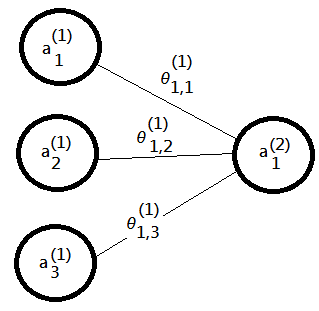
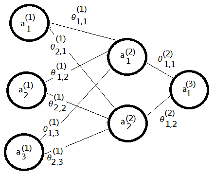
Suppose we are given $3\times1$ neural network model, we know:
➀$z_1^{(2)}=\theta_{1,1}^{(1)}\cdot a_1^{(1)}+\theta_{1,2}^{(1)}\cdot a_2^{(1)}+\theta_{1,3}^{(1)}\cdot a_3^{(1)}$
➁$a_1^{(2)}=g(z_1^{(2)})=\frac1{1+e^{-z_1^{(2)}}}$
➂take partial derivative of $J(\theta)$ on $\theta_{1,1}^{(1)}$, we would obtain:
\(\frac{\partial J(\theta)}{\partial\theta_{1,1}^{(1)}}=\frac{\partial J(\theta)}{\partial a_1^{(2)}}\cdot\frac{\partial a_1^{(2)}}{\partial z_1^{(2)}}\cdot\frac{\partial z_1^{(2)}}{\partial\theta_{1,1}^{(1)}}\)
This is the chain rule in calculus, which would mostly be applied in our later paragraph of proof.
But, why we have the term $\frac{\partial a_1^{(2)}}{\partial z_1^{(2)}}$?
Please be recalled that $a_1^{(2)}=g(z_1^{(2)})$
, where we have below deduction:
\(\begin{array}{l}\frac{\partial J(\theta)}{\partial a_1^{(2)}}=\frac{\partial(-y\cdot\log(a_1^{(2)})-(1-y)\cdot\log(1-a_1^{(2)}))}{\partial a_1^{(2)}}\\\;\;\;\;\;\;\;\;\;\;\;\;\;=\frac{-y}{a_1^{(2)}}+\frac{1-y}{1-a_1^{(2)}}\cdots(a)\\\frac{\partial a_1^{(2)}}{\partial z_1^{(2)}}=\frac{\partial g(z_1^{(2)})}{\partial z_1^{(2)}}=g(z_1^{(2)})\cdot(1-g(z_1^{(2)}))\cdots(b)\\\frac{\partial z_1^{(2)}}{\partial\theta_{1,1}^{(1)}}=a_1^{(1)}\cdots(c)\end{array}\)
Then, combine above (a), (b), (c) terms, we can have:
\(\begin{array}{l}\frac{\partial J(\theta)}{\partial\theta_{1,1}^{(1)}}\\=(a)\cdot(b)\cdot(c)\\=\frac{-y\cdot(1-a_1^{(2)})+(1-y)\cdot a_1^{(2)}}{a_1^{(2)}\cdot(1-a_1^{(2)})}\cdot a_1^{(2)}\cdot(1-a_1^{(2)})\cdot a_1^{(1)}\\=(a_1^{(2)}-y)\cdot a_1^{(1)}\end{array}\)
Continue to apply, we can have results:
\(\left\{\begin{array}{l}\frac{\partial J(\theta)}{\partial\theta_{1,2}^{(1)}}=(a_1^{(2)}-y)\cdot a_2^{(1)}\\\frac{\partial J(\theta)}{\partial\theta_{1,3}^{(1)}}=(a_1^{(2)}-y)\cdot a_3^{(1)}\end{array}\right.\)
Next, we introduce $\delta_j^{(\mathcal l)}$, it is the error cost in $j$-th activation function of layer $\mathcal l$.
With above deduction result, for each distinct input data at index $i$_$data$, we can take error at output layer $2$(in this example):
\(\delta^{(2)}={\begin{bmatrix}\delta_1^{(2)}\end{bmatrix}}_{1\times1}=a_1^{(2)}-y^{(i\_data)}\)
Things would be a little complicated, before this article formularize the gradient computation for each $\frac{\partial J(\theta)}{\partial\theta_{i,j}^{(\mathcal l)}}$, just think that you can compute the errors from the final output layer, in the reversed order, back to the beginning second layer, and the output error from each layer $\mathcal l$ would then be propagated back into the gradient $\frac{\partial J(\theta)}{\partial\theta_{i,j}^{(\mathcal l-1)}}$.
From now on, we are going to do the real proof to formularize the gradient in neural network model:
[1]suppose you can recognize above proof given in $3\times1$ neural network model, and we have the finding:
$$\frac{\partial J(\theta)}{\partial\theta_{i,j}^{(\mathcal l)}}=(a_i^{(\mathcal l+1)}-y^{(i\_data)})\cdot a_j^{(\mathcal l)}=\delta_i^{(\mathcal l+1)}\cdot a_j^{(\mathcal l)}$$
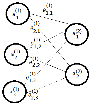
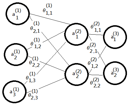
[2]next, we step further into 2 output nodes in final layer, $3\times2$ neural network model:

➀in this case, for $i=1,2$, we can have:
\(a_i^{(2)}=g(z_i^{(2)})=g(\theta_{i,1}^{(1)}\cdot a_1^{(1)}+\theta_{i,2}^{(1)}\cdot a_2^{(1)}+\theta_{i,3}^{(1)}\cdot a_3^{(1)})\)
➁succeeding to the result in [1];, take error costs at layer 2(in this example) as:
\(\delta_{2\times1}^{(2)}={\begin{bmatrix}\delta_1^{(2)}\\\delta_2^{(2)}\end{bmatrix}}_{2\times1}={\begin{bmatrix}a_1^{(2)}-y^{(i\_data)}\\a_2^{(2)}-y^{(i\_data)}\end{bmatrix}}_{2\times1}\)
➂we can deduce out:
\(\begin{array}{l}\frac{\partial J(\theta)}{\partial\theta_{1,1}^{(1)}}=\frac{\partial J(\theta)}{\partial a_1^{(2)}}\cdot\frac{\partial a_1^{(2)}}{\partial z_1^{(2)}}\cdot\frac{\partial z_1^{(2)}}{\partial\theta_{1,1}^{(1)}}\\=(a_1^{(2)}-y^{(i\_data)})\cdot a_1^{(1)}\end{array}\)
\(\therefore\frac{\partial J(\theta)}{\partial\theta_{1,2}^{(1)}}=(a_1^{(2)}-y^{(i\_data)})\cdot a_2^{(1)}\)
\(\therefore\frac{\partial J(\theta)}{\partial\theta_{1,3}^{(1)}}=(a_1^{(2)}-y^{(i\_data)})\cdot a_3^{(1)}\)
\(\therefore\frac{\partial J(\theta)}{\partial\theta_{2,1}^{(1)}}=(a_2^{(2)}-y^{(i\_data)})\cdot a_1^{(1)}\)
\(\therefore\frac{\partial J(\theta)}{\partial\theta_{2,2}^{(1)}}=(a_2^{(2)}-y^{(i\_data)})\cdot a_2^{(1)}\)
\(\therefore\frac{\partial J(\theta)}{\partial\theta_{2,3}^{(1)}}=(a_2^{(2)}-y^{(i\_data)})\cdot a_3^{(1)}\)
By mathematics induction, we have a finding the same as the one in [1]:
$$\frac{\partial J(\theta)}{\partial\theta_{i,j}^{(\mathcal l)}}=(a_i^{(\mathcal l+1)}-y^{(i\_data)})\cdot a_j^{(\mathcal l)}=\delta_i^{(\mathcal l+1)}\cdot a_j^{(\mathcal l)}$$
I have just proved for the simple model of only 2 layers, but, will the current finding hold for models of more than 3 layers?
[3]further step into $3\times2\times1$ neural network model:

➀trivially, we can deduce out that:
\(\delta^{(3)}={\begin{bmatrix}\delta_1^{(3)}\end{bmatrix}}_{1\times1}={\begin{bmatrix}a_1^{(3)}-y^{(i\_data)}\end{bmatrix}}_{1\times1}\)
Then, we have a problem here, what is $\delta^{(2)}$? How to evaluate it? Since it is not at the final layer. What is the gradient descendent evaluation in $\theta^{(1)}$?
➁The same by taking partial derivative of $J(\theta)$:
\(\begin{array}{l}\frac{\partial J(\theta)}{\partial\theta_{1,1}^{(1)}}=\frac{\partial J(\theta)}{\partial a_1^{(3)}}\cdot\frac{\partial a_1^{(3)}}{\partial\theta_{1,1}^{(1)}}\\\end{array}\)
\(\begin{array}{l}=\frac{\partial J(\theta)}{\partial a_1^{(3)}}\cdot(\frac{\partial a_1^{(3)}}{\partial a_1^{(2)}}\cdot\frac{\partial a_1^{(2)}}{\partial z_1^{(2)}}\cdot\frac{\partial z_1^{(2)}}{\partial\theta_{1,1}^{(1)}}\\\end{array}\)
\(\begin{array}{l}+\frac{\partial a_1^{(3)}}{\partial a_2^{(2)}}\cdot\frac{\partial a_2^{(2)}}{\partial z_2^{(2)}}\cdot\frac{\partial z_2^{(2)}}{\partial\theta_{1,1}^{(1)}})\;\cdots\;\frac{\partial z_2^{(2)}}{\partial\theta_{1,1}^{(1)}}=0\\\end{array}\)
\(\begin{array}{l}=\frac{\partial J(\theta)}{\partial a_1^{(3)}}\cdot\frac{\partial g(z_1^{(3)})}{\partial z_1^{(3)}}\cdot\frac{\partial z_1^{(3)}}{\partial a_1^{(2)}}\cdot\frac{\partial a_1^{(2)}}{\partial z_1^{(2)}}\cdot\frac{\partial z_1^{(2)}}{\partial\theta_{1,1}^{(1)}}\\\end{array}\)
\(\begin{array}{l}\cdots\frac{\partial a_1^{(3)}}{\partial a_1^{(2)}}=\frac{\partial g(z_1^{(3)})}{\partial z_1^{(3)}}\cdot\frac{\partial z_1^{(3)}}{\partial a_1^{(2)}}\\\end{array}\)
\(\begin{array}{l}=(a_1^{(3)}-y^{(i\_data)})\cdot\theta_{1,1}^{(2)}\cdot g(z_1^{(2)})\cdot(1-g(z_1^{(2)}))\cdot a_1^{(1)}\\\end{array}\)
\(\therefore\frac{\partial J(\theta)}{\partial\theta_{1,2}^{(1)}}=(a_1^{(3)}-y^{(i\_data)})\cdot\theta_{1,1}^{(2)}\cdot g(z_1^{(2)})\cdot(1-g(z_1^{(2)}))\cdot a_2^{(1)}\)
\(\therefore\frac{\partial J(\theta)}{\partial\theta_{1,3}^{(1)}}=(a_1^{(3)}-y^{(i\_data)})\cdot\theta_{1,1}^{(2)}\cdot g(z_1^{(2)})\cdot(1-g(z_1^{(2)}))\cdot a_3^{(1)}\)
\(\therefore\frac{\partial J(\theta)}{\partial\theta_{2,1}^{(1)}}=(a_1^{(3)}-y^{(i\_data)})\cdot\theta_{1,2}^{(2)}\cdot g(z_2^{(2)})\cdot(1-g(z_2^{(2)}))\cdot a_1^{(1)}\)
\(\therefore\frac{\partial J(\theta)}{\partial\theta_{2,2}^{(1)}}=(a_1^{(3)}-y^{(i\_data)})\cdot\theta_{1,2}^{(2)}\cdot g(z_2^{(2)})\cdot(1-g(z_2^{(2)}))\cdot a_2^{(1)}\)
\(\therefore\frac{\partial J(\theta)}{\partial\theta_{2,3}^{(1)}}=(a_1^{(3)}-y^{(i\_data)})\cdot\theta_{1,2}^{(2)}\cdot g(z_2^{(2)})\cdot(1-g(z_2^{(2)}))\cdot a_3^{(1)}\)
➂we can normalize above result in this given example:
\(\frac{\partial J(\theta)}{\partial\theta_{i,j}^{(\mathcal l)}}=(a_1^{((\mathcal l+1)+1)}-y^{(i\_data)})\cdot\theta_{1,i}^{(\mathcal l+1)}\cdot g(z_i^{(\mathcal l+1)})\cdot(1-g(z_i^{(\mathcal l+1)}))\cdot a_j^{(\mathcal l)}\)
\(\therefore\delta_i^{(\mathcal l+1)}=(a_1^{((\mathcal l+1)+1)}-y^{(i\_data)})\cdot\theta_{1,i}^{(\mathcal l+1)}\cdot g(z_i^{(\mathcal l+1)})\cdot(1-g(z_i^{(\mathcal l+1)}))\)
➃For $\mathcal l=1$, we have error costs at layer two:
\(\delta_i^{(2)}=(a_1^{(3)}-y^{(i\_data)})\cdot\theta_{1,i}^{(2)}\cdot g(z_i^{(2)})\cdot(1-g(z_i^{(2)}))\)
where $i=1,2$, then:
\(\delta_{2\times1}^{(2)}={\begin{bmatrix}\delta_1^{(2)}\\\delta_2^{(2)}\end{bmatrix}}_{2\times1}\)
\(=(a_1^{(3)}-y^{(i\_data)})\cdot{\begin{bmatrix}\theta_{1,1}^{(2)}\\\theta_{1,2}^{(2)}\end{bmatrix}}_{2\times1}.\times\)
\({\begin{bmatrix}g(z_1^{(2)})\cdot(1-g(z_1^{(2)}))\\g(z_2^{(2)})\cdot(1-g(z_2^{(2)}))\end{bmatrix}}_{2\times1}\)
\(\cdots\;.\times\;element-wised\;operator\)
\(\cdots\begin{bmatrix}\theta^{(2)}\end{bmatrix}^t=\begin{bmatrix}\theta_1^{(2)}\\\theta_2^{(2)}\end{bmatrix}\)
\(=(a_1^{(3)}-y^{(i\_data)})\cdot{\begin{bmatrix}\theta_{1,1}^{(2)}\cdot g(z_1^{(2)})\cdot(1-g(z_1^{(2)}))\\\theta_{1,2}^{(2)}\cdot g(z_2^{(2)})\cdot(1-g(z_2^{(2)}))\end{bmatrix}}_{2\times1}\)
By mathematics induction, we have a finding the same as the one in [1]:
$$\frac{\partial J(\theta)}{\partial\theta_{i,j}^{(\mathcal l)}}=(a_i^{(\mathcal l+1)}-y^{(i\_data)})\cdot a_j^{(\mathcal l)}=\delta_i^{(\mathcal l+1)}\cdot a_j^{(\mathcal l)}$$
[4]further step into $3\times2\times2$ neural network model:

➀it would be easy to show error costs at layer three and two:
\(\delta_{2\times1}^{(3)}={\begin{bmatrix}\delta_1^{(3)}\\\delta_2^{(3)}\end{bmatrix}}_{2\times1}={\begin{bmatrix}a_1^{(3)}-y^{(i\_data)}\\a_2^{(3)}-y^{(i\_data)}\end{bmatrix}}_{2\times1}\)
\(\delta_{2\times1}^{(2)}=\begin{bmatrix}\theta^{(2)}\end{bmatrix}_{2\times2}^t\cdot{\begin{bmatrix}\delta^{(3)}\end{bmatrix}}_{2\times1}.\times{\begin{bmatrix}g(z_1^{(2)})\cdot(1-g(z_1^{(2)}))\\g(z_2^{(2)})\cdot(1-g(z_2^{(2)}))\end{bmatrix}}_{2\times1}\)
\(\cdots\;.\times\;element-wised\;operator\)
➁first, evaluate $J(\theta)$ at layer 2, that is take derivation of $J(\theta)$ on $\theta_{i,j}^{(2)}$:
\(\begin{array}{l}\frac{\partial J(\theta)}{\partial\theta_{1,1}^{(2)}}=\frac{\partial J(\theta)}{\partial a_1^{(3)}}\cdot\frac{\partial a_1^{(3)}}{\partial\theta_{1,1}^{(2)}}\\=\frac{\partial J(\theta)}{\partial a_1^{(3)}}\cdot\frac{\partial g(z_1^{(3)})}{\partial z_1^{(3)}}\cdot\frac{\partial z_1^{(3)}}{\partial\theta_{1,1}^{(2)}}\\=(a_1^{(3)}-y^{(i\_data)})\cdot a_1^{(2)}\\=\delta_1^{(3)}\cdot a_1^{(2)}\end{array}\)
\(\begin{array}{l}\therefore\frac{\partial J(\theta)}{\partial\theta_{1,2}^{(2)}}=\delta_1^{(3)}\cdot a_2^{(2)}\\\therefore\frac{\partial J(\theta)}{\partial\theta_{2,1}^{(2)}}=\delta_2^{(3)}\cdot a_1^{(2)}\\\therefore\frac{\partial J(\theta)}{\partial\theta_{2,2}^{(2)}}=\delta_2^{(3)}\cdot a_2^{(2)}\end{array}\)
➂we can by mathematics induction to have error costs at layer two:
\(\frac{\partial J(\theta)}{\partial\theta_{i,j}^2}=\delta_i^{(3)}\cdot a_j^{(2)}\)
➃next, evaluate $J(\theta)$ at layer 1, that is take derivation of $J(\theta)$ on $\theta_{i,j}^{(1)}$:
\(\begin{array}{l}\frac{\partial J(\theta)}{\partial\theta_{1,1}^{(1)}}=\frac{\partial J(\theta)}{\partial a_1^{(3)}}\cdot\frac{\partial a_1^{(3)}}{\partial\theta_{1,1}^{(1)}}+\frac{\partial J(\theta)}{\partial a_2^{(3)}}\cdot\frac{\partial a_2^{(3)}}{\partial\theta_{1,1}^{(1)}}\\=\frac{\partial J(\theta)}{\partial a_1^{(3)}}\cdot\frac{\partial g(z_1^{(3)})}{\partial z_1^{(3)}}\cdot\frac{\partial z_1^{(3)}}{\partial\theta_{1,1}^{(1)}}\\+\frac{\partial J(\theta)}{\partial a_2^{(3)}}\cdot\frac{\partial g(z_2^{(3)})}{\partial z_2^{(3)}}\cdot\frac{\partial z_2^{(3)}}{\partial\theta_{1,1}^{(1)}}\end{array}\)
\(take\;part\;1=\frac{\partial g(z_1^{(3)})}{\partial z_1^{(3)}}\cdot\frac{\partial z_1^{(3)}}{\partial\theta_{1,1}^{(1)}}\)
\(take\;part\;2=\frac{\partial g(z_2^{(3)})}{\partial z_2^{(3)}}\cdot\frac{\partial z_2^{(3)}}{\partial\theta_{1,1}^{(1)}}\)
➄evaluate on $part\;1$:
\(part\;1=\frac{\partial g(z_1^{(3)})}{\partial z_1^{(3)}}\cdot(\frac{\partial z_1^{(3)}}{\partial a_1^{(2)}}\cdot\frac{\partial a_1^{(2)}}{\partial\theta_{1,1}^{(1)}}+\frac{\partial z_1^{(3)}}{\partial a_2^{(2)}}\cdot\frac{\partial a_2^{(2)}}{\partial\theta_{1,1}^{(1)}})\)
\(=\frac{\partial g(z_1^{(3)})}{\partial z_1^{(3)}}\cdot(\theta_{1,1}^{(2)}\cdot\frac{\partial g(z_1^{(2)})}{\partial z_1^{(2)}}\cdot\frac{\partial z_1^{(2)}}{\partial\theta_{1,1}^{(1)}}+\)
\(\theta_{1,2}^{(2)}\cdot\frac{\partial g(z_2^{(2)})}{\partial z_2^{(2)}}\cdot\frac{\partial z_2^{(2)}}{\partial\theta_{1,1}^{(1)}})\cdots\frac{\partial z_2^{(2)}}{\partial\theta_{1,1}^{(1)}}=0\)
\(=\frac{\partial g(z_1^{(3)})}{\partial z_1^{(3)}}\cdot\theta_{1,1}^{(2)}\cdot g(z_1^{(2)})\cdot(1-g(z_1^{(2)}))\cdot a_1^{(1)}\)
Then, evaluate on $part\;2$:
\(part\;2=\frac{\partial g(z_2^{(3)})}{\partial z_2^{(3)}}\cdot(\frac{\partial z_2^{(3)}}{\partial a_1^{(2)}}\cdot\frac{\partial a_1^{(2)}}{\partial\theta_{1,1}^{(1)}}+\frac{\partial z_2^{(3)}}{\partial a_2^{(2)}}\cdot\frac{\partial a_2^{(2)}}{\partial\theta_{1,1}^{(1)}})\)
\(\cdots\frac{\partial a_2^{(2)}}{\partial\theta_{1,1}^{(1)}}=0\)
\(=\frac{\partial g(z_2^{(3)})}{\partial z_2^{(3)}}\cdot\theta_{2,1}^{(2)}\cdot\frac{\partial{g(z_1^{(2)})}}{\partial z_1^{(2)}}\cdot\frac{\partial z_1^{(2)}}{\partial\theta_{1,1}^{(1)}}\)
\(=\frac{\partial g(z_2^{(3)})}{\partial z_2^{(3)}}\cdot\theta_{2,1}^{(2)}\cdot g(z_1^{(2)})\cdot(1-g(z_1^{(2)}))\cdot a_1^{(1)}\)
➅back to the derivation of $J(\theta)$ on $\theta_{i,j}^{(1)}$, at this moment, take $part\;1$, $part\;2$ thus obtained in it:
\(\frac{\partial J(\theta)}{\partial\theta_{1,1}^{(1)}}=\frac{\partial J(\theta)}{\partial a_1^{(3)}}\cdot part\;1+\frac{\partial J(\theta)}{\partial a_2^{(3)}}\cdot part\;2\)
\(=\frac{\partial J(\theta)}{\partial a_1^{(3)}}\cdot\frac{\partial g(z_1^{(3)})}{\partial z_1^{(3)}}\cdot\theta_{1,1}^{(2)}\cdot g(z_1^{(2)})\cdot\)
\(\;\;\;\;\;\;\;\;(1-g(z_1^{(2)}))\cdot a_1^{(1)}\)
\(+\frac{\partial J(\theta)}{\partial a_2^{(3)}}\cdot\frac{\partial g(z_2^{(3)})}{\partial z_2^{(3)}}\cdot\theta_{2,1}^{(2)}\cdot g(z_1^{(2)})\cdot\)
\(\;\;\;\;\;\;\;\;(1-g(z_1^{(2)}))\cdot a_1^{(1)}\)
\(=\delta_1^{(3)}\cdot\theta_{1,1}^{(2)}\cdot g(z_1^{(2)})\cdot(1-g(z_1^{(2)}))\cdot a_1^{(1)}\)
\(+\delta_2^{(3)}\cdot\theta_{2,1}^{(2)}\cdot g(z_1^{(2)})\cdot(1-g(z_1^{(2)}))\cdot a_1^{(1)}\)
\(=\begin{bmatrix}\theta_{1,1}^{(2)}&\theta_{2,1}^{(2)}\end{bmatrix}\cdot\begin{bmatrix}\delta_1^{(3)}\\\delta_2^{(3)}\end{bmatrix}\cdot g(z_1^{(2)})\cdot(1-g(z_1^{(2)}))\cdot a_1^{(1)}\)
\(=\delta_1^{(2)}\cdot a_1^{(1)}\)
➆next, we take $\delta_1^{(2)}$ to be $\begin{bmatrix}\theta_{1,1}^{(2)}&\theta_{2,1}^{(2)}\end{bmatrix}\cdot\begin{bmatrix}\delta_1^{(3)}\\delta_2^{(3)}\end{bmatrix}\cdot g(z_1^{(2)})\cdot(1-g(z_1^{(2)}))$.
Therefore, we have $\frac{\partial J(\theta)}{\partial\theta_{1,2}^{(1)}}=\delta_1^{(2)}\cdot a_2^{(1)}$ and $\frac{\partial J(\theta)}{\partial\theta_{1,3}^{(1)}}=\delta_1^{(2)}\cdot a_3^{(1)}$
➇then, further deduce to have below:
\(\frac{\partial J(\theta)}{\partial\theta_{2,1}^{(1)}}=\begin{bmatrix}\theta_{1,2}^{(2)}&\theta_{2,2}^{(2)}\end{bmatrix}\cdot\begin{bmatrix}\delta_1^{(3)}\\\delta_2^{(3)}\end{bmatrix}\cdot\)
\(g(z_2^{(2)})\cdot(1-g(z_2^{(2)}))\cdot a_1^{(1)}\)
\(=\delta_2^{(2)}\cdot a_1^{(1)}\)
\(\therefore\frac{\partial J(\theta)}{\partial\theta_{2,2}^{(1)}}=\delta_2^{(2)}\cdot a_2^{(1)}\)
\(\therefore\frac{\partial J(\theta)}{\partial\theta_{2,3}^{(1)}}=\delta_2^{(2)}\cdot a_3^{(1)}\)
We found one thing that error costs also has similar scenario:
\(\delta_{2\times1}^{(2)}=\begin{bmatrix}\delta_1^{(2)}\\\delta_2^{(2)}\end{bmatrix}\)
\(=\begin{bmatrix}\theta^{(2)}\end{bmatrix}^t\cdot\delta^{(3)}.\times\begin{bmatrix}g(z_1^{(2)})\cdot(1-g(z_1^{(2)}))\\g(z_2^{(2)})\cdot(1-g(z_2^{(2)}))\end{bmatrix}\)
[5]By mathematics induction, we can claim for both the gradient and the error costs by below formula:
$$\frac{\partial J(\theta)}{\partial\theta_{i,j}^{(\mathcal l)}}=(a_i^{(\mathcal l+1)}-y^{(i\_data)})\cdot a_j^{(\mathcal l)}=\delta_i^{(\mathcal l+1)}\cdot a_j^{(\mathcal l)}$$
$$\delta^{(\mathcal l)}=\begin{bmatrix}\theta^{(\mathcal l)}\end{bmatrix}^t\cdot\delta^{(\mathcal l+1)}.\times\left[\begin{array}{c}g(z^{(\mathcal l)})\end{array}\cdot(1-g(z^{(\mathcal l)}))\right]$$
Cautions must be made that for bias term, $a_j^{(\mathcal l)}=1$, for $j=1$:
\(\frac{\partial J(\theta)}{\partial\theta_{1,1}^{(1)}}=\delta_1^{(2)}\cdot1\); \(\frac{\partial J(\theta)}{\partial\theta_{2,1}^{(1)}}=\delta_2^{(2)}\cdot1\),…
The Backward Propagation Algorithm
Supopose you are comfortable with erro cost in neural network model after deduction by mathemtics induction, this article would guide you through the backward propagation algorithm:
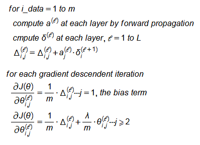
Given the training data set ${(x^{(1)},y^{(1)})\dots(x^{(m)},y^{(m)})}$
Initialize $\triangle_{i,j}^{(\mathcal l)}=0$ for all $i,j,\mathcal l$, below flow is in rather intuition. As to the coding detail, it would be in the impolementation section.

19 Nov 2017
Neural Network Feedforward Propagation
Neural network works as a whole to behave like a perceptron, the output from layer $j$ would be mapped by $\theta^{(j)}$ to the input of layer $j+1$. The final output in last layer would then be classified to
the identity of the target object.
Neural Network Works by Feedforward Propagation
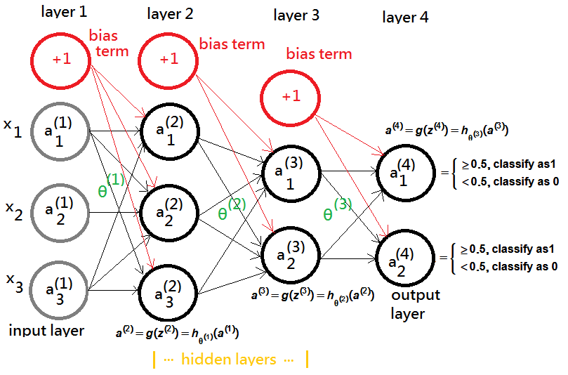
Recap the neural network model:

Note that for the ease of future backpropagation deduction, we further define below formula:
\(\begin{array}{l}a^{(j+1)}=g(z^{(j+1)})=h_{\mathrm\theta^{(\mathrm j)}}(a^{(\mathrm j)})\\,where\;z^{(j+1)}=(\theta^{(j)})^t\cdot a^{(j)},\;g(z)=\frac1{1+e^{-z}}\\\end{array}\)
You can treat g the sigmoid function taking the output($(\theta^{(j)})^t\cdot a^{(j)}$) from prior layer $j$, and transforms it to the input($a^{(j+1)}$) of next layer $j+1$ by means of the logistic regression.
➀from layer 1 to layer 2, we have:
\(\begin{array}{l}a^{(2)}=g(z^{(2)})=h_{\mathrm\theta^{(1)}}(a^{(1)})\\,where\;z^{(2)}=\theta^{(1)}\cdot a^{(1)}\\,a^{(1)}=x^{(i\_data)},1\leq i\_data\leq m\\\end{array}\)
➁from layer 2 to layer 3, we have:
\(\begin{array}{l}a^{(3)}=g(z^{(3)})=h_{\mathrm\theta^{(2)}}(a^{(2)}),where\;z^{(3)}=(\theta^{(2)})^t\cdot a^{(2)}\\\end{array}\)
➂from layer 3 to layer 4, we have:
\(\begin{array}{l}a^{(4)}=g(z^{(4)})=h_{\mathrm\theta^{(3)}}(a^{(3)}),where\;z^{(4)}=(\theta^{(3)})^t\cdot a^{(3)}\\\end{array}\)
➃at the last layer, in this example the layer 4 output, the final identity from logistic regression model would be determined at final layer:
\(\begin{array}{l}a^{(j+1)}=g(z^{(j+1)})=h_{\mathrm\theta^{(j)}}(a^{(j)})=\left\{\begin{array}{l}\geq0.5,clssify\;as\;1\\<0.5,classiy\;as\;0\end{array}\right.\\\end{array}\)
19 Nov 2017
Neural Network Basic Topology
Neural network aims at non-linear hypothesis, binary and multiple classification. In the early 1990, it is believed that it achieves some training hypothesis and come out with results at certain convincible level.
Due to the fact that it was not scaled very well to large problem at theat moment, it has been placed in the storage and it was almost the time I was a freshman in th euniversity. Due to H/W calculation and processing
capability has a major improvement in the past two decads, in conjunction with big data science evolution due to open source environment, neural network has been re-inspected, even more, the deep learning has been build
on top of its model representation. Although his founder Geoff Hilton suspects and claims that backward propagation might not be the most optimal approximation to the way human brain thinking, which is just like
the case that jet engines could make human fly but human couldn't fly like a bird. With full understanding of its model, the way it supports training and recognition would be quiet an add-in in future involve in deep learning.
Model Representation By Intuition
Begin by a very basic realization that human receives external data from eyes, mouth, tongue, skin, then transfer to our brain, wherein, it is manipulated and classified to some other layers or groups of the neurons, which then take their turns to make further processing, maybe neuron transform in a recursive manner. The neural network is constructed with a hope to approximate the way our brain manipulating, training input and learning.

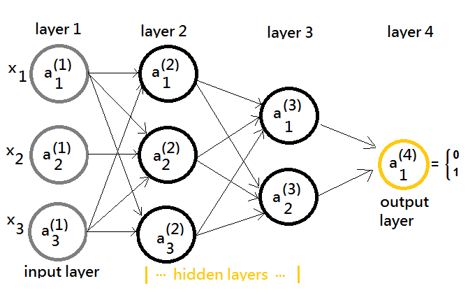
The model representation graph exhibits that there exists an input layer to receive the external data, an output layer to generate the outcome value, some hidden layes(in this example, layer 2, 3) in between the input and the output layer.
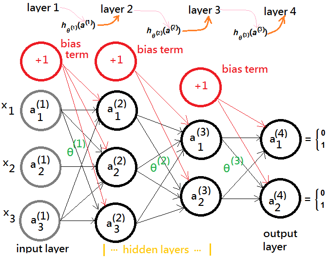
We can have the model more generalized in another graph.

➀you can think of each distinct layer(except for the input layer) in the neural network the individual linear regression model, which (takes an intercept expressed by the bias term by statistics nature design). Specific cares for gradient descendent during backward propagation is mandatory, and the bias term is of no need for regularization!!
➁the $\theta^{(j)}$ is the weighting matrix, controlling the function mapping from layer $j$ to layer $j+1$.
➂the $a_i^{(j)}$ is used to denote the $i$-th activation function at layer $j$, wherein, it takes output from layer $j-1$ as its input and make advanced processing at its layer, output it, in turns becoming the input data to next layer $j+1$.
➃suppose we have the $a_1^{(1)}$, $a_2^{(1)}$,…, $a_n^{(1)}$ as the input data $x\in R^n$.
➄the output from layer $j$(the activation output at layer j) would be mapped to layer $j+1$ by $\theta^{(j)}$ as its input.
➅$h_{\theta^{(j)}}(a^{(j)})$ transforms $a^{(j)}$ with $\theta^{(j)}$ from layer $j$ to layer $j+1$ by means of logistic regression model.
