09 Dec 2019
Prologue To The Chernoff Bounds For Bernoulli Random Variable
The Chernoff bounds is a technique to build the exponential decreasing bounds on tail probabilities. This article develops the tail bound on the Bernoulli random variable with outcome 0 or 1.
The Error Probability After Test
Let $X_{i}$ to be a Bernoulli random variable for $i$=$\{1,2,…,n\}$
➀$X_{i}$=$1$ with probability $p_{i}$
➁$X_{i}$=$0$ with probability $1$-$p_{i}$
, where all $X_{i}$s are I.I.D and suppose at least one of the $p_{i}$ is non-zero.
We are testing with a hope that we can make our target value meet the expectation level after some amount of trials. To express the target value we want in terms of expect value, we let $X$=$\sum_{i=1}^{n}X_{i}$, $E\lbrack X\rbrack$=$\mu$=$\sum_{i=1}^{n}p_{i}$.
[Question]
How confident we are in the final outcome by the random variable $X$? It is asking you 2 kinds of questions:
➀the range of the confidence interval
➁the error probability for the target value $X$ above or below the expect value $\mu$
The follwing section would guide you through the process to build the upper and lower bound of such error probability in Chernoff exponential decreasing form.
[Notes]
Even if our proof of ➁ holds, the range of confidence interval must be guaranteed by the native design in your experiment.
The Upper Bound On Error Probability
It is asking the error probability when target value $X$ is greater than the expect value $\mu$, and we’d like to bound it on the upper side.
$P(X>(1+\delta)\cdot\mu)$, for $\delta>0$
=$P(e^{t\cdot X}>e^{t\cdot (1+\delta)\cdot\mu})$, for all $t>0$
$\leq \frac{E\lbrack e^{t\cdot X}\rbrack}{e^{t\cdot (1+\delta)\cdot\mu}}$…Markov inequality
Since each $X_{i}$ is independent, we have
$E\lbrack e^{t\cdot X}\rbrack$
=$E\lbrack e^{t\cdot \sum_{i=1}^{n}X_{i}}\rbrack$
=$E\lbrack e^{t\cdot (X_{1}+X_{2}+…+X_{n})}\rbrack$
=$E\lbrack \prod_{i=1}^{n} e^{t\cdot X_{i}}\rbrack$
=$\prod_{i=1}^{n} E\lbrack e^{t\cdot X_{i}}\rbrack$
=$\prod_{i=1}^{n} e^{t\cdot 1}\cdot p_{i}+e^{t\cdot 0}\cdot (1-p_{i})$
=$\prod_{i=1}^{n} e^{t}\cdot p_{i}+1\cdot (1-p_{i})$
=$\prod_{i=1}^{n} 1+(e^{t}-1)\cdot p_{i}$
Because $1+X<e^{X}$ for all $X>0$, we have
$E\lbrack e^{t\cdot X}\rbrack$
=$\prod_{i=1}^{n} 1+(e^{t}-1)\cdot p_{i}$
$<\prod_{i=1}^{n} e^{(e^{t}-1)\cdot p_{i}}$
=$e^{(e^{t}-1)\cdot (p_{1}+…+p_{n})}$
=$e^{(e^{t}-1)\cdot\mu}$
Therefore, we have
$P(X>(1+\delta)\cdot\mu)$
$\leq \frac{E\lbrack e^{t\cdot X}\rbrack}{e^{t\cdot (1+\delta)\cdot\mu}}$
$<\frac {e^{(e^{t}-1)\cdot\mu}}{e^{t\cdot (1+\delta)\cdot\mu}}$
=$e^{((e^{t}-1)-t\cdot (1+\delta))\cdot\mu}$…➀
Next would be to figure out the minimum of $e^{((e^{t}-1)-t\cdot (1+\delta))\cdot\mu}$ by taking its first derivative with respect to $t$, set it to zero, get such value of $t$ to make it zero:
$\frac{\operatorname d{e^{((e^{t}-1)-t\cdot (1+\delta))\cdot\mu}}}{\operatorname d{t}}$
=$\lbrack e^{t}-(1+\delta)\rbrack\cdot\mu\cdot e^{\lbrack (e^{t}-1)-(1+\delta)\cdot t\rbrack\cdot\mu}$
The right side of exponential part won’t be zero, then
$\lbrack e^{t}-(1+\delta)\rbrack\cdot\mu$=$0$
$\Rightarrow e^{t}-(1+\delta)$=$0$
$\Rightarrow t$=$ln(1+\delta)$ could we have the minimum value
Take $t$=$ln(1+\delta)$ into ➀, we get:
$P(X>(1+\delta)\cdot\mu)$<${\lbrack\frac {e^{\delta}}{(1+\delta)^{(1+\delta)}} \rbrack}^{\mu}$…[A]
As a result, $(e^{ln(1+\delta)})^{(1+\delta)\cdot\mu}$=$(1+\delta)^{(1+\delta)\cdot\mu}$
The Lower Bound On Error Probability
It is asking the error probability when target value $X$ is less than the expect value $\mu$, and we’d like to bound it on the lower side.
$P(X<(1-\delta)\cdot\mu)$, for $\delta>0$
=$P(-X>-(1-\delta)\cdot\mu)$
=$P(e^{t\cdot (-X)}>e^{t\cdot (-(1-\delta))\cdot\mu})$, for all $t>0$
$\leq \frac{E\lbrack e^{t\cdot (-X)}\rbrack}{e^{t\cdot (-(1-\delta))\cdot\mu)}}$…Markov inequality
Via similar approach, we could have
$P(X<(1-\delta)\cdot\mu)$<${\lbrack\frac {e^{-\delta}}{(1-\delta)^{(1-\delta)}} \rbrack}^{\mu}$…[B]
Bounding The Bounds
We now have 2 bounds in [A] and [B], such bounds ${\lbrack\frac {e^{\delta}}{(1+\delta)^{(1+\delta)}} \rbrack}^{\mu}$ and ${\lbrack\frac {e^{-\delta}}{(1-\delta)^{(1-\delta)}} \rbrack}^{\mu}$ are difficult to use, we should turn it into human readable format.
The nominator is the exponential raised to the power of $\delta$, take upper bound ${\lbrack\frac {e^{\delta}}{(1+\delta)^{(1+\delta)}} \rbrack}^{\mu}$ for illustration, we’d like to turn $(1+\delta)^{(1+\delta)}$ into exponential powered base expression, to be believed the most efficient way.
[1]
The upper bound
Begin from the the natural logarithm of $1+\delta$, that is $ln(1+\delta)$=$y$, then $e^{y}$=$1+\delta$, we can just express $(1+\delta)^{(1+\delta)}$ as $(e^{y})^{(1+\delta)}$, the very next thing would be to figure out $ln(1+\delta)$ in the expression of approximation.
Since $\frac{\operatorname d{ln(1+\delta)}}{\operatorname d{\delta}}$=$\frac {1}{1+\delta}$, the $ln(1+\delta)$ begins from integration:
$ln(1+\delta)$
=$\int_{0}^{1}{\frac {1}{1+\delta}}\operatorname d{\delta}$
=$\int_{0}^{1}{(1-\delta+\delta^{2}-\delta^{3}+\delta^{4}-…)}\operatorname d{\delta}$
=$\delta$-$\frac {\delta^{2}}{2!}$+$\frac {\delta^{3}}{3!}$-$\frac {\delta^{4}}{4!}$+…
=$\sum_{1}^{\infty}(-1)^{k-1}\cdot\frac {\delta^{k}}{k!}$
This $\delta$ is quiet small, temporarily forget about it after the power of 3, then we have
$(1+\delta)^{(1+\delta)}$>$(e^{\delta-\frac {\delta^{2}}{2!}+\frac {\delta^{3}}{3!}})^{(1+\delta)}$
$\;\;\;\;\;\;\;\;\approx e^{\delta+\frac {\delta^{2}}{2}-\frac {\delta^{3}}{6}}$
$\;\;\;\;\;\;\;\;\approx e^{\delta+\frac {\delta^{2}}{2+\varepsilon}}$
Therefore, the upper bound in [A] becomes:
$P(X>(1+\delta)\cdot\mu)$<${\lbrack\frac {e^{\delta}}{(1+\delta)^{(1+\delta)}} \rbrack}^{\mu}$
$\Rightarrow P(X>(1+\delta)\cdot\mu)$<${\lbrack \frac {e^{\delta}}{e^{\delta+\frac {\delta^{2}}{2+\varepsilon}}}\rbrack}^{\mu}$
$\Rightarrow P(X>(1+\delta)\cdot\mu)$<$e^{-\frac {\delta^{2}}{2+\varepsilon}\cdot\mu}$
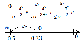
To be more narrow down, the choice of $e^{-\frac {\delta^{2}}{3}\cdot\mu}$ won’t violect, for $\varepsilon\rightarrow 0$:
$\Rightarrow P(X>(1+\delta)\cdot\mu)$<$e^{-\frac {\delta^{2}}{3}\cdot\mu}$
[2]
The lower bound
$ln(1-\delta)$
=$ln(1+(-\delta))$
=$\sum_{1}^{\infty}(-1)^{k-1}\cdot\frac {(-\delta)^{k}}{k!}$
Thus, we have it that
$ln(1-\delta)$=$-\delta-\frac {\delta^{2}}{2!}-\frac {\delta^{3}}{3!}-\frac {\delta^{4}}{4!}-…$
$\Rightarrow ln(1-\delta)$>$-\delta-\frac {\delta^{2}}{2!}$
$\Rightarrow (1-\delta)>e^{-\delta-\frac {\delta^{2}}{2!}}$
$\Rightarrow (1-\delta)^{(1-\delta)}>(e^{-\delta-\frac {\delta^{2}}{2!}})^{(1-\delta)}$
$\Rightarrow (1-\delta)^{(1-\delta)}>e^{-\delta+\frac {\delta^{2}}{2}+\frac {\delta^{3}}{2}}$
$\Rightarrow (1-\delta)^{(1-\delta)}>e^{-\delta+\frac {\delta^{2}}{2}}$, where we ignore the term $\frac {\delta^{3}}{2}$
Therefore, we have the lower bound
$P(X<(1-\delta)\cdot\mu)$<${\lbrack\frac {e^{-\delta}}{(1-\delta)^{(1-\delta)}} \rbrack}^{\mu}$
$\Rightarrow P(X<(1-\delta)\cdot\mu)$<${\lbrack\frac {e^{-\delta}}{e^{-\delta+\frac {\delta^{2}}{2}}} \rbrack}^{\mu}$
$\Rightarrow P(X<(1-\delta)\cdot\mu)$<$e^{-\frac {\delta^{2}}{2}\cdot\mu}$
09 Oct 2019
Prologue To Exploit Evaluation By Hoeffding Bounds
In MDP model, exploration is executed by state transition, exploitation is proceeded by repeating, looping over one node of state. The number of exploitation evaluated by using the Hoeffding bounds would come out the low error result of high probability, pervasively found in modern reinforcement learning.
How Confident We Are In The Seleceted Target Bandit Arm::mjtsai1974
[1]
The question
We are still pulling bandit arm, here is the question, how do we believe that we choose the right bandit? How confident we are in the bandit thus choosed?
[2]
Recap the Chebyshev's inequality
In my prior post Hoeffding Inequality versus Chebyshev’s Inequality, we learn that for any random variable $Y$, the probabilistic error for the differrence in between $Y$ and its expected value $E\lbrack Y\rbrack$ greater than or equal to $\varepsilon$ is smaller than or equal to $\frac {Var\lbrack Y\rbrack}{\varepsilon^{2}}$:
$P(\vert Y-E\lbrack Y\rbrack\vert\geq\varepsilon)\leq\frac {Var\lbrack Y\rbrack}{\varepsilon^{2}}$
Step any further, if we take $X_{i}$ for each distinct $i$-th test, and suppose we believe all $X_{i}$, $i$=$1,2,…,n$ are distributed with expected value $\mu$ and variance $\nu^{2}$, then:
$P(\vert \widehat\mu-\mu\vert\geq\varepsilon)\leq\frac {\nu^{2}}{n\cdot\varepsilon^{2}}$
, where $\widehat\mu$ is the estimator of $\mu$ from all $X_{i}$.
Here we can say the estimator $\widehat\mu$ is bias within $\pm\varepsilon$ is probabilistically less than or equal to $\frac {\nu^{2}}{n\cdot\varepsilon^{2}}$.
The point is how many test cases, how many times we should make the test to convince us that we are confident in this result?
[3]
By using the Hoeffding inequality
My prior post Hoeffding Bounds has proved that it holds for $X_{i}$, $i$=$1,2,…,n$, each weak dependent or identical independent distributed random variables to limit its upper bound:
$P(\vert\sum_{i=1}^{n}(Z_i)\vert\ge n\cdot\varepsilon)\le$ 2$\cdot exp(\frac {-2\cdot n\cdot\varepsilon^2}{(b-a)^2})$
$\Rightarrow P(\vert\sum_{i=1}^{n}(X_i-E\lbrack X_i\rbrack)\vert\ge n\cdot\varepsilon)\le$ 2$\cdot exp(\frac {-2\cdot n\cdot\varepsilon^2}{(b-a)^2})$
$\Rightarrow P(\vert\frac {1}{n}\cdot\sum_{i=1}^{n}(X_i-E\lbrack X_i\rbrack)\vert\ge\varepsilon)\le$ 2$\cdot exp(\frac {-2\cdot n\cdot\varepsilon^2}{(b-a)^2})$
, where
➀$Z_i$=$X_i-E\lbrack X_i\rbrack$ for all $i$
➁$Z_i\in\lbrack a,b\rbrack$
In this Bernoulli bandit arm distribution, we take $a=0$ and $b=1$, the whole average bias of inequality becomes:
$P(\vert\frac {1}{n}\cdot\sum_{i=1}^{n}(X_i-E\lbrack X_i\rbrack)\vert\ge\varepsilon)\le$ 2$\cdot exp(-2\cdot n\cdot\varepsilon^2)$
Now we treat the $i$-th pull of this same bandit arm $X_{i}$=${0,1}$, and take $\widehat u$ to be the average estimated value, take $u$ to be the average expected value, which is the common Hoeffding inequality expression:
$P(\vert \widehat u-u\vert\ge\varepsilon)\le$ 2$\cdot exp(-2\cdot n\cdot\varepsilon^2)$
We could formally claim our bandit arm experiment finally brings us the right arm with the error bias to the true optimal arm limited to $\varepsilon$, which is probabilistically no more than 2$\cdot exp(-2\cdot n\cdot\varepsilon^2)$.
If we choose $\delta$ to be this error of probability, then
$\delta$=2$\cdot exp(-2\cdot n\cdot\varepsilon^2)$
$\Rightarrow \varepsilon$=$(\sqrt {\frac {1}{2}\cdot ln\frac {2}{\delta}})/\sqrt {n}$
$\Rightarrow n$=$(\frac {1}{2}\cdot ln\frac {2}{\delta})/\varepsilon^{2}$
The estimnated $\widehat u$ is probabilistically $1-\delta$ with this precision $[u-\varepsilon,u+\varepsilon]$.
Addendum
➀Exploring Exploration, Charles IsBell, Michael Littman, Reinforcement Learning By Georgia Tech(CS8803)
04 Sep 2019
Prologue To Explore versus Exploit - Part 2
Next would be to get the metrics to construct the fundamental basis of algorithm and validate the bandit arms strategy.
Metrics For Bandit Arm Selection
[1]
Build some metrics
Still we are using the same bandit arms for illustration. To build an algorithm that can make the best bandit arm selection, always a or always b, we need to build some metrics:
➀Identify the optimal bandit arm in the limit.
➁maximize the discounted expected reward.
➂maximize the discounted expected reward over a finite horizon.
➃identify the $\varepsilon$ near optimal arm with high probability $1-\delta$ in the number of steps $T(K,\varepsilon,\delta)$, polynominal in $K$,$\frac {1}{\varepsilon}$,$\frac {1}{\delta}$…[A]
➄find the $\varepsilon$ nearly maximized reward with high probability $1-\delta$ in the number of steps $N(K,\varepsilon,\delta)$, polynominal in $K$,$\frac {1}{\varepsilon}$,$\frac {1}{\delta}$…[B]
➅pull an $\varepsilon$ non-near optimal or near sub-optimal bandit arm with high probability $1-\delta$ in no more than the number of steps $N^{'}(K,\varepsilon,\delta)$ times, polynominal in $K$,$\frac {1}{\varepsilon}$,$\frac {1}{\delta}$…[C]
Above metrics explicitly lead to the construction of reinforcement learning which is the fashion we’d like the algorithm to be executed with, where $K$ is he number of bandit arms.
[2]
Identify the $\varepsilon$ near optimal arm...[A]
➀$\varepsilon$ near optimal doesn't mean that the arm we get is the absolute best arm.
➁we might be unlucky over a long long period and get a pull paid arm. It would be impossible to get the best arm within finite period of time.
For above constraints, what we want with [A] is to get a near optimal arm with only $\varepsilon$ distance from it, it might not workable all the time, but works with hight probability $1-\delta$.
The $T(K,\varepsilon,\delta)$ stands for the number of pulls before we get or have identified the near optimal arm, and it must be polynomial in $K$,$\frac {1}{\varepsilon}$,$\frac {1}{\delta}$.
Indeed, $T(K,\varepsilon,\delta)$ is a polynomial that bounds the number of steps/pulls before we get or have identified the near optimal arm.
[3]
Find the $\varepsilon$ nearly maximized reward...[B]
It is a metric similar to [A], after [B] has been executed over the number of steps $N(K,\varepsilon,\delta)$, we can get the $\varepsilon$ nearly maximized reward.
$N(K,\varepsilon,\delta)$ is the the number of pulls/steps, for which I run that long with [B], I can get $\varepsilon$ nearly maximized reward, with high probability $1-\delta$.
Such number of steps $N(K,\varepsilon,\delta)$ must be polynomial in $K$,$\frac {1}{\varepsilon}$,$\frac {1}{\delta}$.
[B] puts more care on how we reach the optimal arm, not just we get the optimal arm. It focus more directly with rewards, for [A] might do a lot of unfortune trials with zero or a few pay off, we need to evaluate if current accumulated rewards is sufficient to be the incentive to keep going on in the same direction.
[4]
Pull an $\varepsilon$ non-near optimal(naer sub-optimal) arm...[C]
This is a mistake bound. Inevitably, we might pull non-near optimal arm, the mistake arm.
We want to limit the number of pulls of such non-near optimal or sub-optimal arm to $N^{'}(K,\varepsilon,\delta)$, which is a small number.
It could be over a very very long time window, but the number of mistake pulls is really small, with high probability $1-\delta$.
[5]
A brief summary - PAC
➀[A] focus more on identifying the best output, the near optimal arm, the exploitation.
➁[B] is the accumulated return of rewards, which is the exploration.
➂[C] is the mistake bound.
This looks like PAC(Probabily Approximately Correct) learning, some paper refer it PAO(Probabily Approximately Optimal). Even though above metrics are not fully correct, if the goal is to identify the best arm, we could regard it as classification.
The Equilibrium Of Metrics [A] And [B] And [C]
[1]
The target of proof
The very next thing is to prove the transitivity in metrices [A],[B] and [C], that is to say:
$\;\;$Find Best$\Leftrightarrow$Low Mistakes$\Leftrightarrow$Doing Well

[2]
Find Best$\Rightarrow$Low Mistakes
➀the beginning:
Given that you have an algorithm [A] that can identify $\varepsilon$ near optimal arm with high probability $1-\delta$ in the bounded number of pulls $T(K,\varepsilon,\delta)$, polynominal in $K$,$\frac {1}{\varepsilon}$,$\frac {1}{\delta}$.
➁next target:
We’d like to build another algorithm of low mistakes, the number of trials at which it pulls a non $\varepsilon'$ close(mistake) arm is bounded by $T^{'}(K,\varepsilon^{'},\delta^{'})$, where $\varepsilon'\geq\varepsilon$ and is high probability $1-\delta^{'}$.
proof:
$\Rightarrow$first by using algorithm [A], within bounded number of pulls $T(K,\varepsilon,\delta)$, we can find $\varepsilon$ near optimal arm with high probability $1-\delta$.
$\Rightarrow$then, what's the total number of mistakes [A] can make?
Since it is the bounded number of pulls, after that, we can find $\varepsilon$ near optimal arm, that is to say no more than $T(K,\varepsilon,\delta)$.
$T^{'}(K,\varepsilon^{'},\delta^{'})\leq T(K,\varepsilon,\delta)$
$\Rightarrow$why $T'(K,\varepsilon',\delta')$ is the total number of mistakes?
Because the idea of [A] is $\varepsilon$ near optimal arm, and the execution of [A] comes out the non $\varepsilon'$ close(or say $\varepsilon'$ near optimal) arm, where $\varepsilon'\geq\varepsilon$. And we treat the non $\varepsilon'$ close(or say $\varepsilon'$ near optimal) arm as the mistake arm.
$\Rightarrow$we thus prove find best[A]$\Rightarrow$low mistakes[C].
[3]
Low Mistakes$\Rightarrow$Doing Well
➀the beginning:
Given that you have algorithm [C] that bounds the mistake pulls of $\varepsilon$ sub-optimal arms in $T(K,\varepsilon,\delta)$, with high probability $1-\delta$, polynominal in $K$,$\frac {1}{\varepsilon}$,$\frac {1}{\delta}$.
➁next target:
We’d like to build another algorithm that brings you the $\varepsilon'$ nearly maximized reward, in other words, $\varepsilon'$ close to optimal per step reward, with high probability $1-\delta’$, polynominal in $K$,$\frac {1}{\varepsilon’}$,$\frac {1}{\delta’}$.
proof:
$\Rightarrow$first by using algorithm [C], $T(K,\varepsilon,\delta)$ is the upper bound for mistake pulls, beyond this upper bound, you can do a lot pulls of correctness, say $T’(K,\varepsilon’,\delta’)$, take it as $n$, far more than this upper bound.
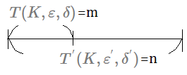
All the rest in $T’(K,\varepsilon’,\delta’)$ beyond $T(K,\varepsilon,\delta)$ have to be $\varepsilon’$ near optimal.
$\Rightarrow$here is one hint to remind you that from the point that you have pulled up to $T(K,\varepsilon,\delta)$ times, do you just start to make the pulls of right arm?
No, it's just [C] constraints the mistake pulls in $T(K,\varepsilon,\delta)$.
At this point, the distance from optimal reward would be greater than $\varepsilon$.
$\Rightarrow$this is a Bernoulli bandit, each pull gives you either zero or one paid. So, if you accumulate mistake pulls up to $T(K,\varepsilon,\delta)$ times, the total fail cases of mistake paid is $T(K,\varepsilon,\delta)\cdot 1$, we take it as $m$. At this moment, it is just $\varepsilon$ close to optimal, bypass the mistakes.
$\Rightarrow$the total sub-optimality over the end, left steps is $m+\varepsilon\cdot(n-m)$. And the average per step sub-optimality is $\frac {m+\varepsilon\cdot(n-m)}{n}$, where this average per step sub-optimality is greater than the distance to the optimal reward, that is to say $\varepsilon’\leq\frac {m+\varepsilon\cdot(n-m)}{n}$. Ideally, we want the distance $\varepsilon'$ optimal is smaller than the distance to the pull of mistake arms.
$\Rightarrow$if we take $\varepsilon$=$\frac {\varepsilon’}{2}$ to try to further narrow down the mistake pulls, above inequality becomes:
$\varepsilon’\geq\frac {m+\frac {\varepsilon’}{2}\cdot(n-m)}{n}$, then
$n\geq m\cdot(\frac {2}{\varepsilon'}-1)$
It is just the quantity that $n$ should have been to make algorithm [B] validate or concrete. We thus prove low mistakes[C]$\Rightarrow$doing well[B].
[4]
Doing Well$\Rightarrow$Find Best
➀the beginning:
Given that you have algorithm [B] that can find the $\varepsilon$ nearly maximized reward, with high probability $1-\delta$, after it has been executed over the number of steps $T(K,\varepsilon,\delta)$, which is polynominal in $K$,$\frac {1}{\varepsilon}$,$\frac {1}{\delta}$.
➁next target:
We want to build an algorithm that can identify $\varepsilon’$ close to optimal arm, with high probability $1-\delta’$, after it has been pulled over $T’(K,\varepsilon’,\delta’)$ times.
proof:
$\Rightarrow$first by using algorithm [B], we do get the $\varepsilon$ nearly maximized reward arm, that’s the per step $\varepsilon$ nearly optimal reward arm.
If we keep following the probability distribution of this pull, I will get the same per step average.
$\Rightarrow$next to introduce $e_{i}$, the sub-optimality for the error of $arm_{i}$, that is you should have selected $arm_{i}$, and you havn’t during the execution of algorithm [C].
Such arm is chosen at least $\frac {1}{K}$ of the time, ideally, we want the error of sub-optimality is as small as possible, so the per step optimality $\varepsilon$ should be greater than or equal to $\frac {1}{K}\cdot e_{i}$, that is $\varepsilon\geq\frac {1}{K}\cdot e_{i}$.
$\Rightarrow$we also want this error of sub-optimality to be smaller than $\varepsilon’$, the distance to the most optimal arm, $\varepsilon’\geq e_{i}$, which is the constraint.
$\varepsilon\geq\frac {1}{K}\cdot e_{i}$…➀
$\varepsilon’\geq e_{i}$…➁
We relate $\varepsilon’$ to $\varepsilon$ by taking $\frac {\varepsilon’}{K}$=$\varepsilon$ in ➀, then ➁ holds, everything just holds.
$\Rightarrow$we just prove doing well[B]$\Rightarrow$find best[A], from the point we are $\varepsilon$ close to optimal reawrd, we can identify $\varepsilon'$ close to most optimal arm, where $\varepsilon'\leq\varepsilon$.
Put It Together
Here we can tell that
➀algorithm [A] is for exploitation, to get better estimate of optimal arm.
➁algorithm [B] is for exploration, to have better rewards.
➂algorithm [C] is a mistake bound.
Put it all together, we know that we need exploration and exploitation interchangeable.
Addendum
➀Exploring Exploration, Charles IsBell, Michael Littman, Reinforcement Learning By Georgia Tech(CS8803)
11 Aug 2019
Prologue To Explore versus Exploit - Part 1
Some reference of articles states that exploration is the topic that separates reinforcement learning from other kinds of machine learning. Exploration is part of fundamental trade off of reinforcement learning.
Begin from K-Armed Bandits
[1]
K-armed bandits
Supposed we are given K-armed bandits, where $K$=$7$ in below exhibition. The bandit has no state transition, all about stochasticity, you pull it, you either get a jackpot, or you don’t get a jackpot.
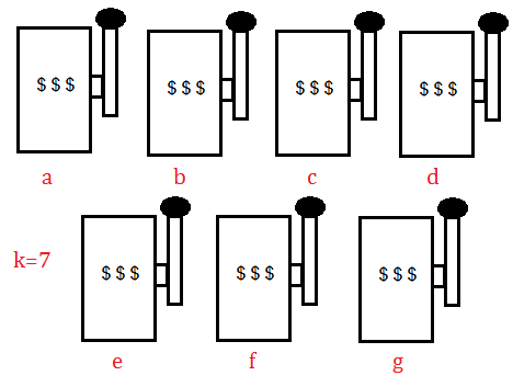
[2]
Which one you will pull?
In this example, suppose each machine will have different paypffs. The question is which bandit will you pull?
➀the one that has the best chance of winning the jackpot, giving you money.
➁the point is that we don’t know the payoffs are, hard to decide which bandit to choose.
➂if we know the payoffs, just do the $max_{arm}Bandit(arm)$ could we get the answer.
[3]
we have to explore
Suppose each bandit has some probability of paying off a one, some probability of paying off nothing, saying that zero. But, we don’t know what it is at first.
If we pull bandit a, and it doesn’t pay off, does it mean that bandit a is not the best one? No, we don’t know what anything else is.
One arm pull just give us some information, but not an awful lot. We have to combine information across a whole lot of pulls to start to evaluate what the best bandit is.
So, we have to explore!!
[4]
Illustration
Suppose each of these bandits has been pulled multiple times and come out the number of times that it pays off 1, with the fomer in the denominator, the later in the nominator, given in below exhibition.
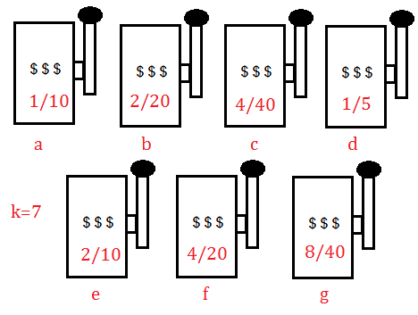 In between a and e, it looks as if that bandit e is better than bandit a, since the same 10 pulls of bandit, e has payed 2 times, while a just 1 time.
Next to examine in between a and d, the bandit d gave the pay off only after 5 pulls, it might also be plausible if we prefer to bandit d rather than a.
By the given data, we have 2 concerns:
➀which bandit is the highest expected pay off?
➁which are we most confident in?
For ➀, the bandits d,e,f,g just play to a tie, since
$\frac {1}{5}\cdot 1$+$\frac {4}{5}\cdot 0$,$\frac {2}{10}\cdot 1$+$\frac {8}{10}\cdot 0$,$\frac {4}{20}\cdot 1$+$\frac {16}{20}\cdot 0$, $\frac {8}{40}\cdot 1$+$\frac {32}{40}\cdot 0$, are the expected pay off for bandit d,e,f,g respectively. They are all the same higher than the rest.
For ➁, as to the confidence level, if you choose g, it might be a good answer, but not the good reason. When it comes to expectation, the confidence level is monotonically increasing function of the numbers of sample. so, whichever has the biggest pulling numbers should be the most confident, because it has most samples. We finally compare c and g, and choose g.
Confidence-Based Exploration
[1]
Something else in stochasticity
Given 2 bandits a and b, you make 1 pull of a and get 0 pay off, whereas, you make 2 pulls of b and get 1 pay off. Do you think the best thing at this point is to always pick up a, always pick up b, or something else?
Trivially, something else.
First, let’s calculate out the probability for:
➀always a to get 0 pay off
$\frac {1}{C_{1}^{3}}\cdot 1$=$\frac {1}{3}$
Since there exists 1 pull of bandit a out of the 3 pulls, and it indeed come out with 0 pay off.
➁always b to get 1 pay off
$\frac {1}{C_{2}^{3}}\cdot 2$=$\frac {2}{3}$
We treat 3 pulls as distinct computation unit, by given, there exists 2 pulls of bandit b and come out with 1 pay off. Totally 2 out of 3 pulls, we prefer all bandit b, where each pull is not replacable, and the 1 pay off might be appeared in the 1st or 2nd pull, that’s why we multiply by 2 at the end.
Suppose you choose bandit b by intuition, you are right $\frac {2}{3}$ of the time, but with $\frac {1}{3}$ of chance you make mistake. That’s why we end up with something else.
[2]
What is something else?
If we run an arbitrary number of pulls, what is something else? I think, we might just evaluate which bandit to pull after some time, or infinite amount of time later. Then, I might know the true expected value for pulling bandit a or b, so I know which to choose.
It refers to the thing I’d like to do to get me more confidence in my expectation, and more number of pulls explicitly. Get more confidence in expectation would be the next step:
➀maximum likelihood
➁maximum confidence level
➂minimum confidence level
[3]
Maximum likelihood
The maximum likelihood over here is to find out the bandit which has the highest expected pay off, and choose it, then keep revisiting this question.
Each time you pull the bandit, recalculate your expected values again and again. choose the highest pay off bandit and continue so on.
As new data of next pull comes in, we will refactor our calculation and make new decision again, but, that’s not a good approach.
By the given case, bandit b is the maximum likelihood, say $MLE_{a}$=$0$,$MLE_{b}$=$0.5$. In this test of maximum likelihood, you will just choose b as beginning, since $MLE_{b}$>$MLE_{a}$.
When I choose b for the very first time, whatever outcome of the result, the expected pay off of b is much higher than bandit a. Next, I continue to choose b, it still has expected pay off higher than 0, such behavior would be elapsed over a long long period would just fall into the expectation. And, it will begin to approach to 0 after an infinite amount of time.
The major point is that even if I choos b and it never pay off, it still has non-zero expected pay off, which implies that I never have the chance to choose a, it is equivalent to say that $\frac {2}{3}$ of the time you are right, but $\frac {1}{3}$ of the time you make mistake.
We can do better than that.
[4]
Maximum confidence level
The maximum confidence level is the strategy for whichever one you have the best estimate, you should choose that one. But, that’s the bad idea, too. Why?
Because whichever one I start out must have the most(current maximum) confidence level of positive result, which implies that I will have more and more data to further consolidate the current maximum confidence one.
Although current maximum confidence level of positive result bandit might not guarantee its future pay off, it still can keep non-zero expected payoff over some period of time. In this example, the strategy will always choose b.
[5]
Minimum confidence level
The minimum confidence level is to choose the bandit of most(current minimum) confidence level of expected payoff.
In this case, you would choose bandit a, if it happens to come out with 1 pay off, that is $P(a)$=$0.5$ and $P(b)$=$0.5$, it just break at a tie. If multiple bandits have the same minimum confidence level, it doesn't matter which one you choose.
What happens, if you choose bandit a, it comes out with 0 pay off?
This strategry would continue to choose the one of minimum confidence level, that is bandit a, until $P(a)$=$P(b)$=$0.5$.
At the moment it plays all bandits to a tie, it just proceeds in the fashion of round robbin. The very next time, when the result is skewed, it will choose the one with the less confidence level, continue and so on.
If you use this strategy, then it will uniformly distributed on all the bandits, and give you the answer to choose any of the bandits.
[6]
There must be something else
So, there must be something else outside maximum likelihood,maximum confidence level,minimum confidence level. These are not better than always a, or always b.
Cautions must be made that the maximum likelihood is not a bad idea, whereas minimum confidence level is not a terrible method, either, for they two bring you the new data.
Some textbooks treat maximum likelihood as exploration, relate minimum confidence level to exploitation:
➀the maximum likelihood gets you more rewards.
➁the minimum confidence level gives you better estimates.
Addendum
➀Exploring Exploration, Charles IsBell, Michael Littman, Reinforcement Learning By Georgia Tech(CS8803)
07 Jul 2019
Prologue To Meshing The Rewards - Part 2
Meshing the reward funtion without impact on the original optimal policy by taking potential(or states of the world) into consideration is the suggestive approach not to struggle over the local suboptimal endless looping.
The Concept Of Potential
Instead of giving static( or fixed) bonus at the moment the state transition has been done, we change to put a little bonus with regards to the states of the world. When you achieve a certain state of the world, you get the bonus, when you unachieve that state of the world, you lose that bonus. Everything balances out nicely.
[mjtsai think]
Step further, such intuition should be aligned with Calculus fashion, when it is in some fixed point and approaching to the target, the value(bonus) should be returned in certain proportion in that fixed point, and this return value varies with respect to per changing from one distincet fixed point to its next, might be in the time unit, or quantity in some scale. Such returned value could be the accumulation in either increasing or descreasing fashion.
[Notes::1]
We want to give hints
Suppose we are design a system of learning agent to make the socker robot to kick the ball into the door.
If we follow up the prior post, the existing official reward function would give us $+100$ for scoring the goal. Now, we might want to give hints to the system about:
➀how close the robot is to the ball
➁the robot is hitting the ball
➂the ball enters the goal
It depends how detail you’d like your design to simulate a physical socker game, maybe
➃how close the ball is to the goal
We need to express ➀,➁,➂,➃ in terms of the states of the world.
[Notes::2]
The potential
As to the MDP states we already know, you can regard it as the fixed state, the value function returns the value(bonus) that is binding in the state, not the state of the world mentioned above.
So, how close the robot is to the ball is the item we’d like to keep track of, we denote it as the potential.
The already know bonus(the reward) obtained after per state transition is left as it is, we’d like to illustrate the way to mesh the reward function by incorporating the factor of potential.
Change-In-State-Based Bonus
[1]
Basic idea
Suppose we are designing the learning agent of socker robot, instead of just giving little bonus as a return every time the robot does a certain thing, we are going to keep track of what the state of the world is.
As we are more close to the state of the world we desire, we are going to obtain reward for it, in contrary to the case we are far away from the state of the world, we are going to lose the reward gained when we are close to this state of the world. Therefore, we should substract the reward off when we move away from those states of the world.
The point is that the change-in-state-based bonus thus obtained would be an increment or decrement in accordance to how close or how far you are subscribed by the state of the world, not the fixed constant.
If the robot is 5 pixels away from the ball to 10 pixels away from the ball, then we might obtain $-5$ of decrement, it depends on how you design, we can also define the bonus as the inverse of distance by $\frac {1}{distance}$, that is to say, if we change from 10 pixels away from the ball to 5 pixels away from the ball, we get $\frac {1}{5}-\frac {1}{10}$=$0.1$; in reverse direction, we lose bonus of $-0.1$.
Such kind of design keeps the account balance in a good shape, it gives positive return as you are approaching the state of world, as you leaves the same state of world, you just lose prior bonus by negating it, you are not just coninue to loop over and over again to get that positive return.
[2]
Change-in-state-based v.s. state-based::mjtsai1974
Here we are about this question how to tell the difference in between change-in-state-based and state-based bonus. If it is a state-based, it returns bonus of fixed value. To reach this state-based point, a sequence of actions might be taken, then we involve change-in-state-based concern, it could also be a state in MDP.
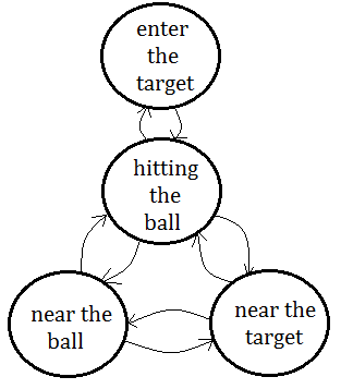
Given that we are developing a robot socker learning agent, the major purpose of the robot is to hit the ball into the target, there must exist a sequence of actions that could be break down:
➀the ball enter into the target, which is the goal of this system
➁the robot should be able to hit the ball
➂the robot should go near the ball
➃the learning agent should evaluate if the ball near the target
I think you can have even more break down items, for the simplicity in this illustration, I come out above 4 items, they are all the already known MDP states.

The point is that we can mesh the reward function by incorporating the potential(the states of world), when the robot is approaching or far away from the ball, the return bonus gets increment or decrement(by negating previous increment). When the ball is near the target, the robot is encouraged by some positive incentive, at the moment the ball is away from the target, the previous returned bonus would be negated and lost.
Above exhibition shows nothing different from already known MDP model. It depends on how you design the learning system. mjtsai think that we should also keep bonus in previous visited states, if we just lose everything learned in current state, at the moment transiting from current to next state, we could not reason for this transition, therefore we should have an appropriate value return as the reward when transiting from current to next state, or such appropriate value might be figured out in accordance to the distance you are away from the ball and that momenmt which you start to speed up to hit the ball.
Potential-Based Shapping: Illustration
[1]
Something we already know
We start from the $Q$ value function already know
$Q(S,A)$=$R(S,A)$+$\gamma\cdot\sum_{S’}P(S’\vert S,A)\cdot max_{A’}Q(S’,A’)$
[2]
add the factor of potential in $R(S,A)$
We take $\psi(S)$ for all $S$ to be the potential:
$R’(S,A,S’)$=$R(S,A)$-$\psi(S)$+$\gamma\cdot\psi(S’)$
, and would like to integrate into the existing Q value function
, next would be the illustration of what the resulting $Q’(S,A)$ in terms of $Q(S,A)$ supposed to be.
[3]
The illustration
➀$Q(S,A)$
=$R(S,A)$+$\gamma\cdot\sum_{S’}P(S’\vert S,A)\cdot max_{A’}Q(S’,A’)$
=$\sum_{S’}P(S’\vert S,A)\cdot R(S,A)$+$\gamma\cdot\sum_{S’}P(S’\vert S,A)\cdot max_{A’}Q(S’,A’)$
=$\sum_{S’}P(S’\vert S,A)\cdot (R(S,A)$+$\gamma\cdot max_{A’}Q(S’,A’))$
, where we departure from $S$ to $S’$, would definitely obtain $R(S,A)$, and the summation over all weighting averaged by the transition probability would finally leads to $1$.
➁$Q’(S,A)$
=$\sum_{S’}P(S’\vert S,A)\cdot (R(S,A,S’)$+$\gamma\cdot max_{A’}Q(S’,A’))$
=$\sum_{S’}P(S’\vert S,A)\cdot (R(S,A)$-$\psi(S)$+$\gamma\cdot\psi(S’)$
$\;\;$+$\gamma\cdot max_{A’}Q’(S’,A’))$
=$\sum_{S’}P(S’\vert S,A)\cdot (R(S,A)$-$\psi(S)$+$\gamma\cdot\psi(S’)$
$\;\;$+$\gamma\cdot (R(S’,A’)$-$\psi(S’)$+$\gamma\cdot\psi(S^{''})$+$max_{A^{''}}Q’(S^{''},A^{''})))$
➂the term $\gamma\cdot\psi(S')$ would be eliminated by the $\gamma\cdot\psi(S')$ contained in $Q'(S',A')$ after it has been further expanded, continue to follow this fashion, we will get all the incoming potential erased.
➃$Q’(S,A)$
=$\sum_{S’}P(S’\vert S,A)\cdot (R(S,A)$-$\psi(S)$+
$\;\;$+$\gamma\cdot max_{A’}Q(S’,A’))$
=$R(S,A)$-$\psi(S)$+$\gamma\cdot max_{A’}Q(S’,A’))$
=$Q(S,A)$-$\psi(S)$
[4]
We still have the same optimal policy
We do still have the same optimal policy after meshing the reward function by means of potential, since $\psi(S’)$ doesn’t depend on $A’$, the term $max_{A’}Q(S’,A’)$ would not be impacted, and we could safely cancel all the incoming $\psi(S)$ term, for all $S$. Even if we reach the convergent point, only one term $\gamma^{n}\cdot \psi(S^{n})$ would be left, and it might be ignored for $n\rightarrow\infty$.
We have shown up that meshing reward function makes no impact on original optimal policy, a lot reference claim that it might do the little help, where mjtsai think that the final term $\gamma^{n}\cdot \psi(S^{n})$ might be the key factor providing small value of very very tiny quantity.
Why such small value could do the help? The answer might be that after such a long term period convergence, equation of potential-based shapping comes out future information(or knowledge) far far away from current time tick, which could be helpful to evaluate if we should take this action!
[5]
A brief review
We have explored 3 total different ways of messaingaround with rewards to give us new $Q$ functions that don't actually change the policy:
➀multiply by $c$, where $c>0$
➁add a constant
➂add this potential function $\psi(S)$ for all $S$
$Q$-Learning With Potentials
[1]
Mesh reward function in $Q$-learning
Above section illustrates meshing the reward functionn by means of potential in the Bellman equation, in this section, we’d like to carry out this potential function idea in the context of $Q$-learning.
$Q_{t+1}(S,A)$
=$Q_{t}(S,A)$+$\alpha_{t}\cdot (R-\psi(S)+\gamma\cdot\psi(S)$
$\;\;$+$\gamma\cdot max_{A’}Q_{t}(S’,A’)-Q_{t}(S,A))$
Suppose you understand this expression of Temporal Difference In Q Form that the state action pair is updated for the state action pair we just left and move a little bit in the direction of the reward plus the discounted value of the state we arrive, minus the value of the state we just left.
This time, we’d like to shift the real reward R around, mesh it with the potential function. So, we take the real reward $R$, substrate the potential we are leaving, and add the discounted potential for the state we end up in.
[2]
What will happen?
If we run above version of $Q$-learning, it should actually solve the original MDP, which is $(R+\gamma\cdot max_{A'}Q_{t}(S',A')-Q_{t}(S,A))$, since $\psi(S)$ doesn’t depend on action.
[3]
What, if $\psi(S)$=$max_{A}Q^{\ast}(S,A)$?
If $\psi(S)$=$max_{A}Q^{\ast}(S,A)$, then it already done, and it’s under the condition that we have solved the MDP problem.
Obviously, the equation becomes
$Q(S,A)$
=$Q^{\ast}(S,A)$-$\psi(S)$
=$Q^{\ast}(S,A)$-$max_{A}Q^{\ast}(S,A)$
We have 2 results:
➀$Q(S,A)=0$ for the optimal action.
➁$Q(S,A)<0$ for some special usage for each action, or by the amount of local sub-optimal.
[4]
Potential function might be helpful
Above results strike on our head that most often we initialize the $Q$ function to all zeros, because we believe zero is where everything starts, or we just know nothing about it.
Such initialization might start to head for the right direction, or it might take some non-optimal action with negative reward, after that just take another better one. This says that Potential function might be helpful in speeding up learning.
[5]
$Q$-learning with or without potential function are the same
Eric Wiewiora has proved potential-based shaping and Q-value initialization are equivalent.
This paper says that the series of updates that you get by running $Q$-learning with some potential function is actually the same as what you get by $Q$-learning without a potential function, on conditions that you should initialize the $Q$ function(without a potential) to what the potential function would have been, that is $Q(S,A)$+$\psi(S)$.
The $Q$ function without potential is initialized as $Q(S,A)$+$\psi(S)$ is different from the $Q$ function with potential in the learning process.
Not only does $Q(S,A)$+$\psi(S)$ converges to the same policy, but also going to have the same policy at every state transition in learning.
$\psi(S)$ is just a constant, it doesn't depend on any action, has no impact on original policy, its shift($Q(S,A)$+$\psi(S)$) has an impact on what the $Q$ values are converging toward.
[6]
$Q$-learning with or without potential function are the same::proof::mjtsai1974
We mesh the reward function by $R(S,A)$-$\psi(S)$+$\gamma\cdot \psi(S’)$, and the potential add-in is refered as $\gamma\cdot \psi(S’)$-$\psi(S)$.
The given $Q$ value function in TD format:
$Q_{t+1}(S,A)$
=$Q_{t}(S,A)$+$\alpha\cdot(R(S,A)+\gamma\cdot max_{A’}Q_{t}(S’,A’)-Q_{t}(S,A))$
First express the $Q$-learning with potential in all state transitions:
$Q_{t+1}(S,A)$
=$Q_{t}(S,A)$+$\alpha\cdot(R(S,A)-\psi(S)+\gamma\cdot\psi(S’)$
$\;\;$+$\gamma\cdot max_{A’}Q_{t}(S’,A’)-Q_{t}(S,A))$…[A]
Next to express the $Q$-learning without potential add-in and initialize the $Q$ value to the potential $\psi(S)$:
$Q_{t+1}^{'}(S,A)$
=$Q_{t}(S,A)$+$\psi(S)$+$\alpha\cdot(R(S,A)$
$\;\;$+$\gamma\cdot max_{A^{'}}Q_{t}^{'}(S^{'},A^{'})-Q_{t}^{'}(S,A))$…[B]
We’d like to prove [A]=[B]
proof::mjtsai1974
➀expand from [B]’s delta part
$\alpha\cdot(R(S,A)$
$\;\;$+$\gamma\cdot max_{A^{'}}Q_{t}^{'}(S^{'},A^{'})-Q_{t}^{'}(S,A))$
=$\alpha\cdot(R(S,A)$
$\;\;$+$\gamma\cdot max_{A^{'}}(Q_{t}(S^{'},A^{'})+\psi(S^{'}))-(Q_{t}(S,A)+\psi(S)))$
=$\alpha\cdot(R(S,A)$+$\gamma\cdot\psi(S^{'})$-$\psi(S)$
$\;\;$+$\gamma\cdot max_{A^{'}}Q_{t}(S^{'},A^{'})-Q_{t}(S,A))$
➁expand from [A]’s delta part
$\alpha\cdot(R(S,A)-\psi(S)+\gamma\cdot\psi(S^{'})$
$\;\;$+$\gamma\cdot max_{A^{'}}Q_{t}(S^{'},A^{'})-Q_{t}(S,A))$
=$\alpha\cdot(R(S,A)+\gamma\cdot\psi(S^{'})-\psi(S)$
$\;\;$+$\gamma\cdot max_{A^{'}}Q_{t}(S^{'},A^{'})-Q_{t}(S,A))$
We found [A] and [B] they two are the same in the delta part.
➂now only the $Q_{t}(S,A)$ in [A] versus $Q_{t}(S,A)$+$\psi(S)$ in [B], where the $\psi(S)$ is the shift added to all the states $S$ in each transition, and it depends on no action, thus no impact on the original optimal policy.
We finally prove that under a broad category of policies, the behavior of these two learners [A] and [B] are indistinguishable.
Potentials Are Just Like Initialization
[1]
The interpretation of potential
We can treat the potential to be $Q$ values initialization.
[2]
Random initialization is debatable
We can make the achievement of potential function by means of $Q$ values initialization, we already encountered, guess what?
➀initialize with all zeros.
➁random initialization.
When you make initialization with all zeros, this might due to the fact that you don’t know anything about it. All zeros initialization might be useful for the scenario that everything begins from zero, but this might not be the true thing in real world.
As to random initialization, you are asserting that these particular(random) values could not be the correct departuring point, you expect these random values to be the right configuration. Then, why not just beginning with the correct initializaton?
[3]
Why not initializedd with the correct value?
One reason for random values might be due to that you don’t know, if you always give it all zeros, or some high values versus low values, you are just biasing it.
You shouldn't be randomly initializing $Q$ functions, basically, you are injecting knowledge!!! But, not noise!!!
Knowledge and noise don’t both start within, only noise does. We could regard noise as the beginning of knowledge.
The punchline is that you shouldn't randomly initialize your $Q$ functions, you can actually inject various kinds of knowledge by $Q$ learning with $\psi(S)$ to be all state $S$'s initialization value.
Cautions must be made that potential function might hurts.
Addendum
➀Meshing with rewards, Charles IsBell, Michael Littman, Reinforcement Learning By Georgia Tech(CS8803)
➁Potential-Based Shaping and Q-Value Initialization are Equivalent, Eric Wiewiora, Department of Computer Science and Engineering University of California, San Diego


 In between a and e, it looks as if that bandit e is better than bandit a, since the same 10 pulls of bandit, e has payed 2 times, while a just 1 time.