13 Dec 2017
SMO Framework And Algorithm
SMO algorithm is the realization of updating mandatory coefficients in the objective function based on the long and tedious deduction with a hope to regularize
by optimization in accordance to the KKT rules that can sequentially costruct the boundarys of the safeguard.
SMO Framework
Let me make a brief summary of the major points from the initial idea to the end of the deduction of the objective function.
[1]Suppose we’d like to have a hyperplane with a safeguard that can classify the given data sample.
➀we formulate our problem as:
$\underset w{min}\frac12w^t\cdot w$, subject to $y_i\cdot(w^t\cdot x_i-b)\geq1,\forall i$.
The first part is the target, the second part is the constraint.
➁then, introduce $\alpha_1,\alpha_2,\dots\alpha_n$ to be the lagrange multiplier and express in below lagrangian to be our objective function:
\(L(w,b,\alpha)=\frac12w^t\cdot w-\sum_{i=1}^n\alpha_i\cdot(y_i\cdot(w^t\cdot x_i-b)-1)\)
➂next to regularize the objective function, to get the optimal $\alpha$, we should take partial derivatives of $L$ on $w$, $b$ respectively and equate them to zero. Finally, we get:
\(\begin{array}{l}L(w,b,\alpha)\\=-\frac12\sum_{i,j=1}^n\alpha_i\cdot\alpha_j\cdot y_i\cdot y_j\cdot(x_i^t\cdot x_j)\\+\sum_{i=1}^n\alpha_i\end{array}\)
where $w=\sum_{i=1}^n\alpha_i\cdot y_i\cdot x_i$.
By such design guarantees that we could have $\forall\alpha_i>0$, one basic condition must be satisfied in SMO.
[2]Next to the imperfect separation with noise. There exists some condition that we don’t strictly enforce that no data points in between $H_1$ and $H_2$. We can extend SVM to allow some noise(data points) in between the safeguard zone. Thus, we want to penalize the data points that cross the boundaries($H_1$,$H_2$).
➀we formulate our problem as:
$\underset{w,\xi_i}{min}\left[w^t\cdot w+C\cdot\sum_{i=1}^n\xi_i\right]$,
subject to
$y_i\cdot(w^t\cdot x_i-b)+\xi_i-1\geq0$, $\forall\xi_i\geq0$
Such design is to shrink down the distance between $H_1$ and $H_2$, thus to allow some noise within original margin.
➁next to build the lagrangian by introducing $\alpha_1$, $\alpha_2$,…, $\alpha_n$ and $\mu_1$, $\mu_2$,…, $\mu_n$, then:
\(\begin{array}{l}L(w,b,\xi,\alpha,\mu)\\=\frac12\cdot w^t\cdot w+C\cdot\sum_{i=1}^n\xi_i\\\;\;\;\;-\sum_{i=1}^n\alpha_i\cdot(y_i\cdot(w^t\cdot x_i-b)+\xi_i-1)\\\;\;\;\;-\sum_{i=1}^n\mu_i\cdot\xi_i\end{array}\)
The lagrangian expression turns out to be:
\(\begin{array}{l}L(w,b,\xi,\alpha,\mu)\\=\frac12\cdot w^t\cdot w+\sum_{i=1}^n(C-\alpha_i-\mu_i)\xi_i\\\;\;\;\;-\sum_{i=1}^n(\alpha_i\cdot y_i\cdot x_i^t)\cdot w\\\;\;\;\;+\sum_{i=1}^n\alpha_i\cdot y_i\cdot b\\\;\;\;\;+\sum_{i=1}^n\alpha_i\end{array}\)
➂to get the maximum of $L$ at $\alpha$ and $\xi$, below constraints must be satisfied for all $i$:
$\frac{\partial L}{\partial w}=0$, $\frac{\partial L}{\partial b}=0$, $\frac{\partial L}{\partial \xi}=0$.
We have $w=\sum_{i=1}^n(\alpha_i\cdot y_i\cdot x_i)$, $\sum_{i=1}^n\alpha_i\cdot y_i=0$,
and $\sum_{i=1}^nC-\alpha_i-\mu_i=0$, for all $i$, $C-\alpha_i-\mu_i=0$ just holds.
➃to maximize $L(w,b,\xi,\alpha,\mu)$ for the optimal $\alpha_i$ value, then, we formulate the lagrangian as:
\(\begin{array}{l}\underset\alpha{min}L(w,b,\xi,\alpha,\mu)\\=\sum_{i=1}^n\alpha_i-\frac12\cdot\sum_{i,j=1}^n\alpha_i\cdot\alpha_j\cdot y_i\cdot y_j\cdot x_i^t\cdot x_j\end{array}\)
, subject to $\sum_{i=1}^n\alpha_i\cdot y_i=0$ and $0\leq\alpha_i\leq C$ for all $i$
➄Notes that $\alpha_i\geq0$, $\mu_i\geq0$, therefore, we have $0\leq\alpha_i\leq C$,
$\alpha_i$ is now upper bounded by $C$.
[3]Then, we make introduction to the KKT conditions:
➀$\alpha_i=0$, $R_i\geq0$
➁$0<\alpha_i<C$, $R_i\approx0$
➂$\alpha_i=C$, $R_i\leq0$
Above KKT cases are evaluated by below constraints under $0\leq\alpha_i\leq C$:
➀$\frac{\partial L}{\partial \xi}=C-\alpha_i-\mu_i=0$
➁$\alpha_i\cdot(y_i\cdot(w^t\cdot x_i-b)+\xi_i-1)=0$
Also, we give the KKT violating cases:
➀$\alpha_i<C$ and $R_i<0$
➁$\alpha_i>0$ and $R_i>0$
➂$\alpha_i=0$ and $R_i>0$…by mjtsai
[4]Departure from noise
So far, we have our objective function as:
\(\begin{array}{l}L(w,b,\xi,\alpha,\mu)\\=\sum_{i=1}^n\alpha_i-\frac12\cdot\sum_{i,j=1}^n\alpha_i\cdot\alpha_j\cdot y_i\cdot y_j\cdot x_i^t\cdot x_j\end{array}\)
for all i, $0<\alpha_i<C$, the non-boundary case.
[5]Works on 2 $\alpha$’s at a time
The algorithm of SMO works by manipulating 2 $\alpha$'s at a time(with others fixed), a little hill climbing alike approach. By heuristics to choose 2 $\alpha$’s at a time.
To optimize $\alpha_1$, $\alpha_2$ with other $\alpha$'s fixed, the objective function could be rewritten as:
\(\begin{array}{l}L(w,b,\xi,\alpha,\mu)\\=\alpha_1+\alpha_2+const\\-\frac12\cdot(part\;1+par\;2)\end{array}\)
All deduction is based on below equality:
$\alpha_1+S\cdot \alpha_2=const$,
$\alpha_1=const-S\cdot \alpha_2$,
where $\alpha_1+S\cdot \alpha_2=\alpha_1^{old}+S\cdot \alpha_2^{old}$.
[6]Express $\alpha_1$ in terms Of $\alpha_2$
The major purpose is to express the objective function in terms of single $\alpha_2^{new}$, this is quiet a paintful process.
We’d like to toss out almost everything non-related with $\alpha_2^{new}$ and put it it the $const$ term. The objective function becomes:
\(\begin{array}{l}L(w,b,\xi,\alpha,\mu)\\=\frac12\cdot(2K_{12}-K_{11}-K_{22})\cdot(\alpha_2^{new})^2\\\;\;\;\;+(1-S+S\cdot K_{11}\cdot r-S\cdot K_{12}\cdot r\\\;\;\;\;+y_2\cdot V_1-y_2\cdot V_2)\cdot\alpha_2^{new}\end{array}\)
[7]Transform from $L(w,b,\xi,\alpha,\mu)$ to $L(\alpha_2^{new})$
The major spirit of SMO is to optimize 2 $\alpha$’s at a time, by transiting from the old $\alpha$’s to the new $\alpha$’s, more precisely, from $\alpha_1^{old}$ to $\alpha_1^{new}$, and from $\alpha_2^{old}$ to $\alpha_2^{new}$. First, we focus on $\alpha_2^{new}$, and laterly, get the $\alpha_1^{new}$ after we get $\alpha_2^{new}$.
➀relate $\alpha_2^{new}$ Back To $\alpha_2^{old}$
➁introduction Of $\eta$ by taking $\eta=2K_{12}-K_{11}-K_{22}$, $\eta\leq0$ is the validity of $\eta$.
Now, we formularize our problem in objective function of $\eta$, $\alpha_2^{new}$, $\alpha_2^{old}$, $E_1^{old}$, $E_2^{old}$:
\(\begin{array}{l}L(w,b,\xi,\alpha,\mu)\\=L(\alpha_2^{new})\\=\frac12\cdot\eta\cdot(\alpha_2^{new})^2\\\;\;\;\;+(y_2\cdot(E_1^{old}-E_2^{old})-\eta\cdot\alpha_2^{old})\cdot\alpha_2^{new}\\\;\;\;\;+const\end{array}\)
It is much simpler in its optimization, only $\alpha_2^{new}$ is left to be optimized.
[8]Examine the feasible rangle of new $\alpha$ value
For computation, $\eta$ should be less than $0$
, although it might be approaching to $0$. We have the new $\alpha_2$ expressed in below:
\(\alpha_2^{new}=\alpha_2^{old}+\frac{y_2\cdot(E_2^{old}-E_1^{old})}\eta\)
Then, the $\alpha_2^{new}$ thus obtained might be unconstrainted maximum value. The feasible range of $\alpha_2^{new}$ must be checked.
Take the minimum feasible of $\alpha_2^{new}$ be L, the maximum feasible of $\alpha_2^{new}$ be H, then:
\(\alpha_2^{new,clipped}=\left\{\begin{array}{l}L,if\;\alpha_2^{new}<L\\\alpha_2^{new},if\;L<\alpha_2^{new}<H\\H,if\;\alpha_2^{new}>H\end{array}\right.\)
We can finally go to clip the new $\alpha_1$, $\alpha_2$ value with sequantial updating in $b$ and $w$.
Take $\triangle\alpha_2=\frac{y_2\cdot(E_2^{old}-E_1^{old})}\eta$
Recall that $\alpha_1=r-S\cdot \alpha_2$, it holds for both new and old. Therefore,
\(\lim_{\triangle\rightarrow0}\frac{(\alpha_1+\triangle)-\triangle}\triangle=\lim_{\triangle\rightarrow0}\frac{r-S\cdot(\alpha_2+\triangle)-(r-S\cdot\alpha_2)}\triangle\)
\(\Rightarrow\triangle\alpha_1=-S\cdot\lim_{\triangle\rightarrow0}\frac{(\alpha_2+\triangle)-\alpha_2}\triangle\)
\(\Rightarrow\triangle\alpha_1=-S\cdot\triangle\alpha_2\)
, where $\triangle\alpha_1$, $\triangle\alpha_2$ are the differentials or derivatives of $\alpha_1$, $\alpha_2$.
This is a quiet tedious, complicated process, but a beautiful framework!!
SMO Algorithm
We all have been given the concept that SMO is the process by randomly picking 2 $\alpha$’s at a time, such behavior is called SMO heuristics. The implementation or even algorithm flow could be found the existence of a lot variety. In this section, I’d like to review the algorithm in SMO original design. By usual, you can find one outer loop and one inner loop in the whole flow.
[First heuristic]
It is the outer loop for $\alpha_1$.
➀iterates all training set, if an example is examined as KKT violated; it is eligible for optimization.
➁search the entire training set for non-boundary examples, whose $\alpha\neq0$, $\alpha\neq C$, and $0<\alpha<C$; if such example was found, it is treated as KKT violated, it is eligible for optimization.
➂keep seraching non-boundary examples, until all non-boundary examples obey KKT conditions within $\varepsilon=0.001$.
Where non-boundary case guarantees:
$\left|(w^{new})^t\cdot x_i-y_i\right|\leq\varepsilon$
, for $i=1,2$, and $\varepsilon$ is a rather tiny quantity.
By above ➀, ➁, ➂, examples at boundary are likely to stay at boundary; examples at non-boundary are likely to move toward boundary as they have been optimized.
Why?
Because iteration focus on non-boundary cases and $\alpha_1^{new}=\alpha_1-S\cdot \triangle\alpha_2$ will move this example($\alpha_1^{new}$) toward boundary.
➃after ➀, ➁, ➂ completed, SMO algorithm will start to search boundary case and optimize it if the case has been KKT violated due to non-boundary subset optimization.
[Second heuristic]
It is the inner loop for $\alpha_2$.
Once $\alpha_1$ has been chosen, $\alpha_2$ would be chosen based on the criteria to maximize the step size in each iteration:
$\underset{i,j}{max}\left|E_i-E_j\right|$, where $i$, $j$ would be $1$, $2$. why?
Because it could speed up the converge from non-boundary location to the boundary side, where:
➀$\alpha_2^{new}=\alpha_2^{old}+\frac{y_2\cdot(E_2^{old}-E_1^{old})}\eta$;
➁$\alpha_1^{new}=\alpha_1-S\cdot \triangle\alpha_2$
Before the ending of SVM algorithm, positive progress means from $0<\alpha_i<C$ to $\alpha_i\rightarrow0$ or $\alpha_i\rightarrow C$. From the non-boundary case, then, back to whole training set for optimization by random pick.
At the end, this article would like to remind that not all iteration makes positive progress, if $x_i=x_j$, then $\eta=0$!!! Skip to other case is the recommendation from some code snippet.
07 Dec 2017
Inside Sequential Minimal Optimization
SMO(Sequential Minimal Optimization) is the regularization process by optimization in accordance to the rule that can minimize the cost error of the objective function sequentially.
Departure With Noise
We’d like to begin from the imperfect separation, since no sampling is fully qualified and could be well separated. Given the support vector formulated problem expressed in terms of $\alpha_i$, $y_i$, $x_i$; then the objective function:
\(\begin{array}{l}L(w,b,\xi,\alpha,\mu)\\=\sum_{i=1}^n\alpha_i-\frac12\cdot\sum_{i,j=1}^n\alpha_i\cdot\alpha_j\cdot y_i\cdot y_j\cdot x_i^t\cdot x_j\end{array}\)
for all i, $0<\alpha_i<C$, the non-boundary case.
Works On 2 $\alpha$’s At A Time
The algorithm of SMO works by manipulating 2 $\alpha$'s at a time(with others fixed), a little hill climbing alike approach. By heuristics to choose 2 $\alpha$’s at a time.
In the begin of the whole flow, initialize $\alpha_i=0$ for $i=1$ to $n$. Suppose we randomly choose $\alpha_1$, $\alpha_2$ and denote it as $\alpha_1^{old}$, $\alpha_2^{old}$.
Due to $\sum_{i=1}^n\alpha_i\cdot y_i=0$, therefore we have:
$y_1\cdot \alpha_1+y_2\cdot \alpha_2=y_1\cdot \alpha_1^{old}+y_2\cdot \alpha_2^{old}$
This confines the optimization of $\alpha_1$, $\alpha_2$ is on a line.
Next to examine the relation in between of these 2 $\alpha_1$, $\alpha_2$ of old or new.
➀for $y_1\neq y_2$, then, $\alpha_1-\alpha_2=r$, where $r$ is a constant.
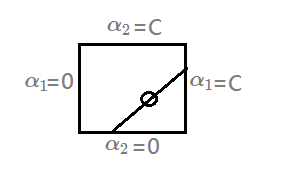 ➁for $y_1=y_2$, then, $\alpha_1+\alpha_2=r$.
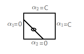 Take $S=y_1\cdot y_2$, multiply $y_1\cdot \alpha_1+y_2\cdot \alpha_2=const$ by $y_1$, then,
$\alpha_1+S\cdot \alpha_2=const$, we have:
$\alpha_1=const-S\cdot \alpha_2$,
where $\alpha_1+S\cdot \alpha_2=\alpha_1^{old}+S\cdot \alpha_2^{old}$.
Next to optimize $\alpha_1$, $\alpha_2$ with other $\alpha$'s fixed, the objective function could be rewritten as:
\(\begin{array}{l}L(w,b,\xi,\alpha,\mu)\\=\alpha_1+\alpha_2+const\\-\frac12\cdot(part\;1+par\;2)\end{array}\)
➀we further express $part\;1$:
\(\begin{array}{l}part\;1\\=\sum_{i,j=1,2}\alpha_i\cdot\alpha_j\cdot y_i\cdot y_j\cdot x_i^t\cdot x_j\\=\alpha_1^2\cdot y_1^2\cdot x_1^t\cdot x_1\\\;\;+\alpha_2^2\cdot y_2^2\cdot x_2^t\cdot x_2\\\;\;+2\cdot\alpha_1\cdot\alpha_2\cdot y_1\cdot y_2\cdot x_1^t\cdot x_2\end{array}\)
➁we express $part\;2$ as:
\(\begin{array}{l}part\;2\\=\sum_{i=3;j=1,2}^{j=n}\alpha_i\cdot\alpha_j\cdot y_i\cdot y_j\cdot x_i^t\cdot x_j\\\;\;+\sum_{i=1,2;j=3}^{j=n}\alpha_i\cdot\alpha_j\cdot y_i\cdot y_j\cdot x_i^t\cdot x_j\\=2\cdot(\sum_{i=3}^n\alpha_i\cdot y_i\cdot x_i^t)\cdot(\alpha_1\cdot y_1\cdot x_1+\alpha_2\cdot y_2\cdot x_2)\end{array}\)
Express $\alpha_1$ In Terms Of $\alpha_2$
Next to express $\alpha_1$ in terms of $\alpha_2$, this is a quiet painful and confused process, it took me some while, now I’d like to share you with my viewpoint in each step in the deduction.
From current objective function, some symptoms could be found that $x_i$ is associasted with $x_j$.
Thus, we take $K_{11}=x_1^t\cdot x_1$, $K_{22}=x_2^t\cdot x_2$, $K_{12}=x_1^t\cdot x_2$.
Recall that it is deduced out by removing the old $\alpha_1$, $\alpha_2$ associated terms from the term $w$, here comes the question, can we relate the old $w$ to the new evolved $\alpha_1$, $\alpha_2$?
\(\begin{array}{l}V_j=\sum_{i=3}^n\alpha_i\cdot y_i\cdot x_i^t\cdot x_j\\=(w^{old})^t\cdot x_j-\alpha_1^{old}\cdot y_1\cdot x_1^t\cdot x_j\\\;\;\;\;-\alpha_2^{old}\cdot y_2\cdot x_2^t\cdot x_j\\=(w^{old})^t\cdot x_j-b^{old}+b^{old}\\\;\;\;\;-\alpha_1^{old}\cdot y_1\cdot x_1^t\cdot x_j\\\;\;\;\;-\alpha_2^{old}\cdot y_2\cdot x_2^t\cdot x_j\\=U_j+b^{old}\\\;\;\;\;-\alpha_1^{old}\cdot y_1\cdot x_1^t\cdot x_j\\\;\;\;\;-\alpha_2^{old}\cdot y_2\cdot x_2^t\cdot x_j\end{array}\)
where $U_j=(w^{old})^t\cdot x_j-b^{old}$ is the output of $x_j$ under the old parameters, $w^{old}$, $b^{old}$. Expression in this way with a hope to refine original objective function.
In order to make it the point, the subscript of the term indicates the index, usually in this proof, they are $i$,$j$ or $1$,$2$…, the superscript is ued for the identity of old or new clipped term.
For the simplicity of the deduction and understanding, if no any word like old, new in the superscript, then, the term is treated as new term. Why by default is the term of new version? Because the nature design in SMO algorithm works by clipping 2 new terms of $\alpha$’s at a time, the objective function would then be refined as the expression of 2 new terms of $\alpha$’s.
➀deduce by replacing above terms in the objective function:
\(\begin{array}{l}L(w,b,\xi,\alpha,\mu)=\alpha_1+\alpha_2+const-\frac12\cdot(\\\;\;\;\;K_{11}\cdot\alpha_1^2+K_{22}\cdot\alpha_2^2+2\cdot S\cdot K_{12}\cdot\alpha_1\cdot\alpha_2+\\\;\;\;\;2\cdot\alpha_1\cdot y_1\cdot V_1+2\cdot\alpha_2\cdot y_2\cdot V_2)\end{array}\)
➁next to replace $\alpha_1$ with $\alpha_2$, more precisely, replace the new $\alpha_1$ with the new $\alpha_2$:
\(\begin{array}{l}=(r-S\cdot\alpha_2)+\alpha_2+const\\\;\;\;\;-\frac12\cdot(K_{11}\cdot(r-S\cdot\alpha_2)^2+K_{22}\cdot\alpha_2^2+\\\;\;\;\;2\cdot S\cdot K_{12}\cdot(r-S\cdot\alpha_2)\cdot\alpha_2+\\\;\;\;\;2\cdot y_1\cdot V_1\cdot(r-S\cdot\alpha_2)+2\cdot\alpha_2\cdot y_2\cdot V_2)\end{array}\)
➂toss out the $r$ in the term $(r-S\cdot\alpha_2)$(or we just put it in the term $const$), since it is just a constant and no association with it, as to the $r$ associated in the remaining terms, it should be retained.
\(\begin{array}{l}=(1-S)\cdot\alpha_2+const\\\;\;\;\;-\frac12\cdot(K_{11}\cdot(r-S\cdot\alpha_2)^2+K_{22}\cdot\alpha_2^2+\\\;\;\;\;2\cdot S\cdot K_{12}\cdot(r-S\cdot\alpha_2)\cdot\alpha_2+\\\;\;\;\;2\cdot y_1\cdot V_1\cdot(r-S\cdot\alpha_2)+2\cdot\alpha_2\cdot y_2\cdot V_2)\end{array}\)
➃expand in terms of $\alpha_2$:
\(\begin{array}{l}=(1-S)\cdot\alpha_2+const\\\;\;\;\;-\frac12\cdot K_{11}\cdot r^2+K_{11}\cdot r\cdot S\cdot\alpha_2-\frac12\cdot K_{11}\cdot S^2\cdot\alpha_2^2\\\;\;\;\;-\frac12\cdot K_{22}\cdot\alpha_2^2\\\;\;\;\;-S\cdot K_{12}\cdot r\cdot\alpha_2+S^2\cdot K_{12}\cdot\alpha_2^2\\\;\;\;\;-y_1\cdot V_1\cdot r+y_1\cdot V_1\cdot S\cdot\alpha_2-y_2\cdot V_2\cdot\alpha_2\end{array}\)
➄since we’d like to express $\alpha_1$ in terms of $\alpha_2$ in the new evolved objective function, it might be a good idea to put the $r$ non-associated with $\alpha_2$ into the $const$ term, where $S^2=1$ and the $-\frac12\cdot K_{11}\cdot r^2$, $-y_1\cdot V_1\cdot r$ should be tossed out:
\(\begin{array}{l}=(1-S)\cdot\alpha_2+const\\\;\;\;\;+K_{11}\cdot r\cdot S\cdot\alpha_2-\frac12\cdot K_{11}\cdot S^2\cdot\alpha_2^2\\\;\;\;\;-\frac12\cdot K_{22}\cdot\alpha_2^2\\\;\;\;\;-S\cdot K_{12}\cdot r\cdot\alpha_2+S^2\cdot K_{12}\cdot\alpha_2^2\\\;\;\;\;+y_1\cdot V_1\cdot S\cdot\alpha_2-y_2\cdot V_2\cdot\alpha_2\end{array}\)
➅it seems that the objective function has been well refined with only $\alpha_2$ in it, but, take a look at the term $y_1\cdot V_1\cdot S\cdot\alpha_2$, it consists of $y_1$ and $\alpha_2$, whereas, $y_1$ is the signal of $\alpha_1$, and $\alpha_2$ should be associated with $y_2$, here comes the tricky factor $S=y_1\cdot y_2$:
\(\begin{array}{l}y_1\cdot V_1\cdot S\cdot\alpha_2\\=y_1\cdot V_1\cdot y_1\cdot y_2\cdot\alpha_2\\=V_1\cdot y_2\cdot\alpha_2\end{array}\)
where $y_1^2=1$, thus, the regularized objective function in this paragraph would be:
\(\begin{array}{l}=(1-S)\cdot\alpha_2+const\\\;\;\;\;+K_{11}\cdot r\cdot S\cdot\alpha_2-\frac12\cdot K_{11}\cdot S^2\cdot\alpha_2^2\\\;\;\;\;-\frac12\cdot K_{22}\cdot\alpha_2^2\\\;\;\;\;-S\cdot K_{12}\cdot r\cdot\alpha_2+S^2\cdot K_{12}\cdot\alpha_2^2\\\;\;\;\;+y_2\cdot V_1\cdot\alpha_2-y_2\cdot V_2\cdot\alpha_2\end{array}\)
➆now, we save with only the $\alpha_2^{new}$ and $(\alpha_2^{new})^2$ are left:
\(\begin{array}{l}=\frac12\cdot(2K_{12}-K_{11}-K_{22})\cdot(\alpha_2^{new})^2\\\;\;\;\;+(1-S+S\cdot K_{11}\cdot r-S\cdot K_{12}\cdot r\\\;\;\;\;+y_2\cdot V_1-y_2\cdot V_2)\cdot\alpha_2^{new}\end{array}\)
Relate $\alpha_2^{new}$ Back To $\alpha_2^{old}$
The major spirit of SMO is to optimize 2 $\alpha$’s at a time, by transiting from the old $\alpha$’s to the new $\alpha$’s, more precisely, from $\alpha_1^{old}$ to $\alpha_1^{new}$, and from $\alpha_2^{old}$ to $\alpha_2^{new}$. Now, we focus on $\alpha_2^{new}$, and laterly, by the relationship in between these 2 $\alpha$’s:
➀$\alpha_1+\alpha_2=r$
➁$\alpha_1-\alpha_2=r$
above equality holds for both the old $\alpha$’s to the new $\alpha$’s, we can get the $\alpha_1^{new}$ after we get $\alpha_2^{new}$.
To link $\alpha_2^{new}$ back to $\alpha_2^{old}$ ,we start below procedure.
➀now, we focus on the coefficient of $\alpha_2^{new}$, expand from $r$ and $V_1$ and $V_2$:
\(\begin{array}{l}1-S+S\cdot K_{11}\cdot r-S\cdot K_{12}\cdot r+y_2\cdot V_1-y_2\cdot V_2\\=1-S+S\cdot K_{11}\cdot(\alpha_1^{old}+S\cdot\alpha_2^{old})\\\;\;\;\;-S\cdot K_{12}\cdot(\alpha_1^{old}+S\cdot\alpha_2^{old})\\\;\;\;\;+y_2\cdot(U_1^{old}+b^{old}-\alpha_1^{old}\cdot y_1\cdot K_{11}-\alpha_2^{old}\cdot y_2\cdot K_{12})\\\;\;\;\;-y_2\cdot(U_2^{old}+b^{old}-\alpha_1^{old}\cdot y_1\cdot K_{12}-\alpha_2^{old}\cdot y_2\cdot K_{22})\end{array}\)
➁further expand:
\(\begin{array}{l}=1-S+S\cdot K_{11}\cdot\alpha_1^{old}+S\cdot K_{11}\cdot S\cdot\alpha_2^{old}\\\;\;\;\;-S\cdot K_{12}\cdot\alpha_1^{old}-S\cdot K_{12}\cdot S\cdot\alpha_2^{old}\\\;\;\;\;+y_2\cdot U_1^{old}+y_2\cdot b^{old}-y_2\cdot\alpha_1^{old}\cdot y_1\cdot K_{11}-y_2\cdot\alpha_2^{old}\cdot y_2\cdot K_{12}\\\;\;\;\;-y_2\cdot U_2^{old}-y_2\cdot b^{old}+y_2\cdot\alpha_1^{old}\cdot y_1\cdot K_{12}+y_2\cdot\alpha_2^{old}\cdot y_2\cdot K_{22}\end{array}\)
➂eliminate these terms $S\cdot K_{11}\cdot \alpha_1^{old}$, $S\cdot K_{12}\cdot \alpha_1^{old}$ and $y_2\cdot b^{old}$:
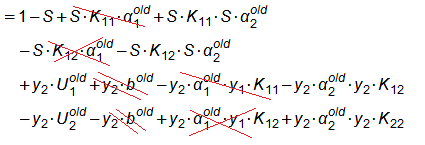 ➃we obtain below equality:
\(\begin{array}{l}=1-S+(K_{11}-2\cdot K_{12}+K_{22})\cdot\alpha_2^{old}\\\;\;\;\;+y_2\cdot(U_1^{old}-U_2^{old})\end{array}\)
, where $U_j^{old}=(w^{old})^t\cdot x_j-b^{old}$.
➄enrich the equation with terms that is related to $\alpha_2$ might be helpful:
\(\begin{array}{l}=(y_2)^2-y_1\cdot y_2+(K_{11}-2\cdot K_{12}+K_{22})\cdot\alpha_2^{old}\\\;\;\;\;+y_2\cdot(U_1^{old}-U_2^{old})\end{array}\)
, where $(y_2)^2=1$ and $y_1\cdot y_2=S$.
Introduction Of $\eta$
Take a look at above ➄, there exists a term $(K_{11}-2\cdot K_{12}+K_{22})$ quiet similar with the term $(2K_{12}-K_{11}-K_{22})$, which is the coefficient of the term $(\alpha_2^{new})^2$.
Next is to further refine the objective funection by introducing $\eta$.
Take $\eta=2K_{12}-K_{11}-K_{22}$, then, the above ➄ becomes:
\(\begin{array}{l}=(y_2)^2-y_1\cdot y_2-\eta\cdot\alpha_2^{old}\\\;\;\;\;+y_2\cdot(U_1^{old}-U_2^{old})\end{array}\)
\(=y_2\cdot(y_2-y_1+U_1^{old}-U_2^{old})-\eta\cdot\alpha_2^{old}\)
\(=y_2\cdot(U_1^{old}-y_1-(U_2^{old}-y_2))-\eta\cdot\alpha_2^{old}\)
\(=y_2\cdot(E_1^{old}-E_2^{old})-\eta\cdot\alpha_2^{old}\)
where $E_1^{old}=Err_{(x_1,y_1)}^{old}=(w^{old})^t\cdot x_1-b^{old}-y_1$,
and $E_2^{old}=Err_{(x_2,y_2)}^{old}=(w^{old})^t\cdot x_2-b^{old}-y_2$.
They are just the error caused by the $w^{old}$, when $\alpha_1^{old}$ and $\alpha_2^{old}$ in it.
Now, we formularize our problem in objective function of $\eta$, $\alpha_2^{new}$, $\alpha_2^{old}$, $E_1^{old}$, $E_2^{old}$:
\(\begin{array}{l}L(w,b,\xi,\alpha,\mu)\\=L(\alpha_2^{new})\\=\frac12\cdot\eta\cdot(\alpha_2^{new})^2\\\;\;\;\;+(y_2\cdot(E_1^{old}-E_2^{old})-\eta\cdot\alpha_2^{old})\cdot\alpha_2^{new}\\\;\;\;\;+const\end{array}\)
Transform from $L(w,b,\xi,\alpha,\mu)$ to $L(\alpha_2^{new})$ is much simpler in its optimization
, since, only $\alpha_2^{new}$ is left to be optimized, the regularization cost of computation is greatly reduced!!!
Now we come to the validity of $\eta$, to get the most optimal vale of $\alpha_2^{new}$:
➀$\frac{\partial L}{\partial\alpha_2^{new}}=\eta\cdot\alpha_2^{new}+y_2\cdot(E_1^{old}-E_2^{old})-\eta\cdot\alpha_2^{old}=0$
➁$\frac{\partial L}{\partial{(\alpha_2^{new})^2}}=\frac12\cdot\eta$, where we have $\eta=2K_{12}-K_{11}-K_{22}$.
By ➀, this coincides with our departure point in the section relate $\alpha_2^{new}$ back to $\alpha_2^{old}$, we just make the point. We have:
\(\alpha_2^{new}=\alpha_2^{old}-\frac{y_2\cdot(E_1^{old}-E_2^{old})}\eta\)
Further refine, we can have:
\(\alpha_2^{new}=\alpha_2^{old}+\frac{y_2\cdot(E_2^{old}-E_1^{old})}\eta\)
$\eta\leq0$ is the validity of $\eta$
and must hold:
\(\begin{array}{l}\eta=2\cdot K_{12}-K_{11}-K_{22}\\\;\;\;=-\left\|x_1-x_2\right\|^2\leq0\end{array}\)
For computation, $\eta$ should be less than $0$
, although it might be approaching to $0$.
Feasible Rangle Of New $\alpha$ Value
Suppose we are working under $\eta<0$ in this equality, and it is correct:
\(\alpha_2^{new}=\alpha_2^{old}+\frac{y_2\cdot(E_2^{old}-E_1^{old})}\eta\)
Then, the $\alpha_2^{new}$ thus obtained might be unconstrainted maximum value. The feasible range of $\alpha_2^{new}$ must be checked.
We’d like to examine 4 cases, begin from below 3 equality:
➀$S=y_1\cdot y_2$.
➁$\alpha_1^{old}+S\cdot \alpha_2^{old}=r=\alpha_1^{new}+S\cdot \alpha_2^{new}$.
➂$0\leq\alpha_i\leq C$, this should be inequality.
[Case 1]$S=1$, $\alpha_1+\alpha_2=r$, $r>C$, then, max($\alpha_2$)=$C$, min($\alpha_2$)=$r-C$
[Case 2]$S=1$, $\alpha_1+\alpha_2=r$, $r<C$, then, max($\alpha_2$)=$r$, min($\alpha_2$)=$0$
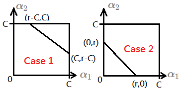 Where the case 1 and case 2 are found to have $y_1=y_2$, we’d like to get the low threshold by max($0$, $r-c$), denote it as L; the hight threshold by min($r$, $C$), denote it as H.
[Case 3]$S=-1$, $\alpha_1-\alpha_2=r$, $r>0$, then, max($\alpha_2$)=$C-r$, min($\alpha_2$)=$0$
[Case 4]$S=-1$, $\alpha_1-\alpha_2=r$, $r<0$, then, max($\alpha_2$)=$C$, min($\alpha_2$)=$-r$
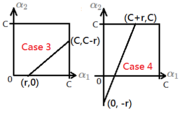 Where the case 3 and case 4 are found to have $y_1\neq y_2$, we’d like to get the low threshold by max($0$, $-r$), denote it as L; the hight threshold by min($C$, $C+r$), denote it as H.
Take the minimum feasible of $\alpha_2^{new}$ be L, the maximum feasible of $\alpha_2^{new}$ be H, then:
\(\alpha_2^{new,clipped}=\left\{\begin{array}{l}L,if\;\alpha_2^{new}<L\\\alpha_2^{new},if\;L<\alpha_2^{new}<H\\H,if\;\alpha_2^{new}>H\end{array}\right.\)
Clip New $\alpha$
Succeeding to above section, in this paragraph, I’d like to summarize the process to clip $\alpha_2^{new}$, then, $\alpha_1^{new}$.
Begin by given $y_1$, $y_2$, $K_{11}$, $K_{22}$, $K_{12}$, $E_1^{old}$, $E_2^{old}$, where $E_i^{old}=w^{old}\cdot x_i-b^{old}-y_i$.
➀take $\eta=2\cdot K_{12}-K_{11}-K_{22}$, then $\eta\leq 0$ must hold.
➁if $\eta<0$, by prior induction, we have:
\(\alpha_2^{new}=\alpha_2^{old}+\frac{y_2\cdot(E_2^{old}-E_1^{old})}\eta\)
Take $\triangle\alpha_2=\frac{y_2\cdot(E_2^{old}-E_1^{old})}\eta$
Please recall that $\alpha_1=r-S\cdot \alpha_2$, it holds for both new and old. Therefore,
\(\lim_{\triangle\rightarrow0}\frac{(\alpha_1+\triangle)-\triangle}\triangle=\lim_{\triangle\rightarrow0}\frac{r-S\cdot(\alpha_2+\triangle)-(r-S\cdot\alpha_2)}\triangle\)
\(\Rightarrow\triangle\alpha_1=-S\cdot\lim_{\triangle\rightarrow0}\frac{(\alpha_2+\triangle)-\alpha_2}\triangle\)
\(\Rightarrow\triangle\alpha_1=-S\cdot\triangle\alpha_2\)
, where $\triangle\alpha_1$, $\triangle\alpha_2$ are the differentials or derivatives of $\alpha_1$, $\alpha_2$.
➂if $\eta=0$, most SMO dosument, just commends to evaluate the objective function at the 2 end points and set $\alpha_2^{new}$ to the one that can make the larger objective function, thus, $\alpha_2^{new}$ would be more closed to boundary!!!
Recap the objective function is now:
\(\begin{array}{l}L(\alpha_2^{new})\\=\frac12\cdot\eta\cdot(\alpha_2^{new})^2\\\;\;\;\;+(y_2\cdot(E_1^{old}-E_2^{old})-\eta\cdot\alpha_2^{old})\cdot\alpha_2^{new}\\\;\;\;\;+const\end{array}\)
Where mjtsai think, for $\eta=0$, alternative would be to abandom and switch to next set of 2 points, since the current evaluated 2 points might just be the duplicated or the overlapped cases(Coursera, M.L professor ANG’s SMO sample code does this).
As to the mirrored case, should keep them in the mutual exclusive list for later manipulation, once new iteration would like to choose the new 2 candidates, already paired 2 points should not be paired again, also by mjtsai.
SMO Updating
We now have the concept that $\alpha_1^{new}$, $\alpha_2^{new}$ are updated by $\triangle\alpha_1$, $\triangle\alpha_2$, this section would like to guide you to update $E_i$, $F_i$, $w$ and $b$.
[Updating $b$]
Take $E(x,y)=\sum_{i=1}^n\alpha_i\cdot y_i\cdot\ x_i^t\cdot x-y-b$ to be the predict error:
$\triangle E(x,y)=\triangle\alpha_1\cdot y_1\cdot x_1^t\cdot x+\triangle\alpha_2\cdot y_2\cdot x_2^t\cdot x-\triangle b$ just holds to be the change in $E$.
If $0<\alpha_1^{new}<C$, then, we can treat the new value of $E_1$ be zero, that is $E_1^{new}=0$, since it is not the boundary case. Recall in the KKT case 2, it is not at boundary, we have $R_i=y_i\cdot E_i=0$. Thus, we can reinforce the new value of $E$ to be $0$.
$E(x,y)$
$=E(x,y)^{old}+\triangle E(x,y)$
$=E(x,y)^{old}+\triangle\alpha_1\cdot y_1\cdot x_1^t\cdot x+\triangle\alpha_2\cdot y_2\cdot x_2^t\cdot x-\triangle b$
$=0$
Then, we have $\triangle b$ in below expression:
\(\triangle b=E(x,y)^{old}+\triangle\alpha_1\cdot y_1\cdot x_1^t\cdot x+\triangle\alpha_2\cdot y_2\cdot x_2^t\cdot x\)
Take $\triangle b=b^{new}-b^{old}$, then:
\(b^{new}=E(x,y)^{old}+\triangle\alpha_1\cdot y_1\cdot x_1^t\cdot x+\triangle\alpha_2\cdot y_2\cdot x_2^t\cdot x+b^{old}\)
We can further deduce out that:
\(b_1^{new}=E(x_1,y_1)^{old}+\triangle\alpha_1\cdot y_1\cdot x_1^t\cdot x_1+\triangle\alpha_2\cdot y_2\cdot x_2^t\cdot x_1+b^{old}\)
\(b_2^{new}=E(x_2,y_2)^{old}+\triangle\alpha_1\cdot y_1\cdot x_1^t\cdot x_2+\triangle\alpha_2\cdot y_2\cdot x_2^t\cdot x_2+b^{old}\)
where
\(\triangle b_1=b_1^{new}-b^{old}\)
\(\triangle b_2=b_2^{new}-b^{old}\)
➀when $\alpha_1^{new}$ (and, or, $\alpha_2^{new}$) is not at boundary, $0<\alpha_1^{new},\alpha_2^{new}<C$, by above deduction, we have $E(x_i,y_i)^{new}=0$, for $i=1,2$, that is to say:
\(R_i=y_i\cdot E_i^{new}=y_i\cdot ((w^{new})^t\cdot x_i-b-y_i)\approx0\)
it holds for $y_i=\pm$, therefore, there should be no change in $b$, we can treat $\triangle b=0$.
$\triangle b=0$
$\;\;\;\;=b_1^{new}-b_1^{old}$
$\;\;\;\;=b_2^{new}-b_2^{old}$, further proof of this:
let $b_1^{new}$, $b_2^{new}$ the bias term after iteration
$(w^{new})^t\cdot x_1-b_1^{new}\approx0$
$(w^{new})^t\cdot x_2-b_2^{new}\approx0$, where non-boundary case guarantees:
$\left|(w^{new})^t\cdot x_i-y_i\right|\leq\varepsilon$
, for $i=1,2$, and $\varepsilon$ is a rather tiny quantity.
therefore, $\varepsilon-b_1^{new}\approx\varepsilon-b_2^{new}$
hence, we have $b_1^{new}\approx b_2^{new}$ as the result.
➁when $\alpha_1^{new}$, $\alpha_2^{new}$ are all at different boundary, one at $0$, one at $C$, where $L\neq H$, then, the interval in between $b_1^{new}$ and $b_2^{new}$ are all constrained by the KKT case 1 and 3, respectively.
Be recalled that KKT case 1 has it that $\alpha_i=0$, $R_i\geq0$; and KKT case 3 has it that $\alpha_i=C$, $R_i\leq0$, the intersection with KKT case 2 is the equality of $0$, $R_i\approx0$, to reinforce these 2 points entering into the support vector, we can just come out with $E(x,y)^{new}=0$. Therefore, we take $b^{new}=\frac{b_1^{new}+b_2^{new}}{2}$, such that the next $b^{new}$ would be stable in this way, the very next time, for current evaluated or other points to be iterated over, it would be much easier to move toward the boundary than current.
On our way to update $b$, in the meanwhile, we update $E_i$.
[Updating $F_i$]
We have it that:
$F(x,y)$
$=w^t\cdot x-y$
$=\sum_{i=1}^{n}\alpha_i\cdot y_i\cdot x_i^t\cdot x-y$
Trivially, we also have it that:
$\triangle F(x,y)$
$=\triangle\alpha_1\cdot y_1\cdot x_1^t\cdot x+\triangle\alpha_2\cdot y_2\cdot x_2^t\cdot x$
[Updating $w$]
Under the assumption that we are using linear kernel,
begin from $w=\sum_{i=1}^{n}\alpha_i\cdot y_i\cdot x_i$,
we can have it that:
$\triangle w=\triangle\alpha_1\cdot y_1\cdot x_1+\triangle\alpha_2\cdot y_2\cdot x_2$
06 Dec 2017
Imperfect Separation And KKT Condition
How, if there exists some data points in the safeguard zone? When we are studying the field of SVM, it is the condition never be abandoned. This article will lead you break through the noise case and come out to the KKT condition.
Imperfect Separation With Noise
There exists some condition that we don’t strictly enforce that no data points in between $H_1$ and $H_2$. We can extend SVM to allow some noise(data points) in between the safeguard zone. Thus, we want to penalize the data points that cross the boundaries($H_1$,$H_2$).
[1]In this way, by introducting $\xi\geq0$, non-negative, such that:
➀$w^t\cdot x_i-b\geq1-\xi_i$, for $y_i=1$
➁$w^t\cdot x_i-b\leq-1+\xi_i$, for $y_i=-1$
This is to shrink down the distance between $H_1$ and $H_2$, thus to allow some noise within original margin.
[2]In addition to $\xi$, we also introduce the penalty $C$, where $C$ is finite in the objective function:
$\underset{w,\xi_i}{min}\left[w^t\cdot w+C\cdot(\sum_{i=1}^n\xi_i)^m\right]$, by usual $m=1$, which then leads to formulate our problem as:
$\underset{w,\xi_i}{min}\left[w^t\cdot w+C\cdot\sum_{i=1}^n\xi_i\right]$,
subject to
$y_i\cdot(w^t\cdot x_i-b)+\xi_i-1\geq0$, $\forall\xi_i\geq0$
[3]Next to build the lagrangian by introducing $\alpha_1$, $\alpha_2$,…, $\alpha_n$ and $\mu_1$, $\mu_2$,…, $\mu_n$, then:
\(\begin{array}{l}L(w,b,\xi,\alpha,\mu)\\=\frac12\cdot w^t\cdot w+C\cdot\sum_{i=1}^n\xi_i\\\;\;\;\;-\sum_{i=1}^n\alpha_i\cdot(y_i\cdot(w^t\cdot x_i-b)+\xi_i-1)\\\;\;\;\;-\sum_{i=1}^n\mu_i\cdot\xi_i\end{array}\)
; where the regularization terms are explained below:
➀the term $y_i\cdot(w^t\cdot x_i-b)+\xi_i-1$ is regularized by $\alpha_i$.
➁$\mu_i$ is for the regularization of the term $\xi_i$.
The lagrangian expression turns out to be:
\(\begin{array}{l}L(w,b,\xi,\alpha,\mu)\\=\frac12\cdot w^t\cdot w+\sum_{i=1}^n(C-\alpha_i-\mu_i)\xi_i\\\;\;\;\;-\sum_{i=1}^n(\alpha_i\cdot y_i\cdot x_i^t)\cdot w\\\;\;\;\;+\sum_{i=1}^n\alpha_i\cdot y_i\cdot b\\\;\;\;\;+\sum_{i=1}^n\alpha_i\end{array}\)
[4]To get the maximum of $L$ at $\alpha$ and $\xi$, below constraints must be satisfied for all $i$:
➀$\frac{\partial L}{\partial w}=0$, ➁$\frac{\partial L}{\partial b}=0$, ➂$\frac{\partial L}{\partial \xi}=0$, for all $i$:
➀we have $w$ in below expression:
\(\begin{array}{l}w^t-\sum_{i=1}^n(\alpha_i\cdot y_i\cdot x_i^t)=0\\\Leftrightarrow w=\sum_{i=1}^n(\alpha_i\cdot y_i\cdot x_i)\end{array}\)
➁implies $\sum_{i=1}^n\alpha_i\cdot y_i=0$
➂we have $\sum_{i=1}^nC-\alpha_i-\mu_i=0$, then for all $i$, $C-\alpha_i-\mu_i=0$ just holds.
[5]Notes that $\alpha_i\geq0$, $\mu_i\geq0$, therefore, we have $0\leq\alpha_i\leq C$,
$\alpha_i$ is now upper bounded by $C$.
[6]Substituting ➀, ➁, ➂ to $L(w,b,\xi,\alpha,\mu)$, then, we have:
\(\begin{array}{l}L(w,b,\xi,\alpha,\mu)\\=\frac12\cdot w^t\cdot w+\sum_{i=1}^n0\cdot\xi_i\\\;\;\;\;-w^t\cdot w+0\cdot b\\\;\;\;\;+\sum_{i=1}^n\alpha_i\\=\sum_{i=1}^n\alpha_i-\frac12\cdot w^t\cdot w\\=\sum_{i=1}^n\alpha_i-\frac12\cdot\sum_{i,j=1}^n\alpha_i\cdot\alpha_j\cdot y_i\cdot y_j\cdot x_i^t\cdot x_j\end{array}\)
[7]To maximize $L(w,b,\xi,\alpha,\mu)$ for the optimal $\alpha_i$ value, then, we formulate the lagrangian as:
\(\begin{array}{l}\underset\alpha{min}L(w,b,\xi,\alpha,\mu)\\=\sum_{i=1}^n\alpha_i-\frac12\cdot\sum_{i,j=1}^n\alpha_i\cdot\alpha_j\cdot y_i\cdot y_j\cdot x_i^t\cdot x_j\end{array}\)
, subject to:
➀$\sum_{i=1}^n\alpha_i\cdot y_i=0$
➁$0\leq\alpha_i\leq C$ for all $i$
Introduction To The KKT Condition
[1]The KKT optimality conditions of the formula in our problem are:
➀the gradient of $L(w,b,\xi,\alpha,\mu)$ with respect to $w$, $b$, $\xi$ vanish, $\frac{\partial L}{\partial w}=0$, ➁$\frac{\partial L}{\partial b}=0$, ➂$\frac{\partial L}{\partial \xi}=0$
➁$\alpha_i\cdot(y_i\cdot(w^t\cdot x_i-b)+\xi_i-1)=0$
➂$\mu_i\cdot\xi_i=0$
where ➁+➂ guarantees that $\xi$ will have the smallest impact on $(w^t\cdot x_i-b)-1$.
[2]By KKT conditions, there exists 3 cases to be evaluated by below constraints:
➀$\frac{\partial L}{\partial \xi}=C-\alpha_i-\mu_i=0$
➁$\alpha_i\cdot(y_i\cdot(w^t\cdot x_i-b)+\xi_i-1)=0$
from which, this paragraph would guide you through the deduction process.
[3]Remember that we have $0\leq\alpha_i\leq C$ for all $i$.
[case 1]$\alpha_i=0$, then, we are at the boundary:
$\mu_i=C-\alpha_i=C>0$, by $\mu_i\cdot\xi_i=0$, we have $\xi_i=0$, thus,
$y_i\cdot(w^t\cdot x_i-b)-1\geq0$
just holds.
[case 2]$0<\alpha_i<C$, the case of non-boundary.
then, $\mu_i=C-\alpha_i>0$, by $\mu_i\cdot\xi_i=0$, again, we have $\xi_i=0$, then,
$y_i\cdot(w^t\cdot x_i-b)+\xi_i-1=0$,
therefore, $y_i\cdot(w^t\cdot x_i-b)-1=0$.
[case 3]$\alpha_i=C$, also, the boundary case.
then, $\mu_i=C-\alpha_i=0$, by $\mu_i\cdot\xi_i=0$, we have $\xi_i\geq0$, then,
$y_i\cdot(w^t\cdot x_i-b)+\xi_i-1=0$,
$y_i\cdot(w^t\cdot x_i-b)-1\leq0$ just holds, more precisely, it should be:
$y_i\cdot(w^t\cdot x_i-b)-1\leq-\xi_i$…by mjtsai
[4]Continue the deduction on the condition term to be regularized by $\alpha_i$ in the most original objective function.
$y_i\cdot(w^t\cdot x_i-b)-1$
$=y_i\cdot(w^t\cdot x_i-b)-y_i^2$
$=y_i\cdot((w^t\cdot x_i-b)-y_i)$
$=y_i\cdot E_i$…$E_i=u_i-y_i$
$=R_i$…$u_i=w^t\cdot x_i-b$
Let’s summarize the KKT conditions:
➀$\alpha_i=0$, $R_i\geq0$
➁$0<\alpha_i<C$, $R_i\approx0$
➂$\alpha_i=C$, $R_i\leq0$
[5]Below lists the KKT violating cases:
➀$\alpha_i<C$ and $R_i<0$
➁$\alpha_i>0$ and $R_i>0$
➂$\alpha_i=0$ and $R_i>0$…by mjtsai
Checking The KKT Without Using Threshold $b$
Due to the fact that $L(w,b,\xi,\alpha,\mu)$ doesn’t solve for $b$ directly, as a result, it would be beneficial to check KKT without using threshold $b$.
$R_i$…begin from here
$=y_i\cdot E_i$
$=y_i\cdot(w^t\cdot x_i-b-y_i)$
$=y_i\cdot(u_i-y_i)$
$=y_i\cdot(w^t\cdot x_i-y_i-b)$
$=y_i\cdot(F_i-b)$…$F_i=w^t\cdot x_i-y_i$
therefore, we have $E_i=F_i-b$, then to evaluated by
$E_i-E_j=F_i-b-(F_j-b)=F_i-F_j$
05 Dec 2017
Value Iteration Algorithm Detail
An optimal policy maps each distinct state to an optimal action maximizing the value of the state over the horizon of some magnitude or even infinity. With an optimal policy, it's easy to evaluate the expected value from each possible starting state by executing it. All above must be resorted to value iteration.
Value Iteration Algorithm/Flow
Let me try to express value iteration flow in below in this section.
Initialize $V_0(S)=0$ for all $S$.
Loop until $\left|V_t-V_{t-1}\right|<\varepsilon\cdot\frac{1-\gamma}\gamma$
Loop for all $S$
\[V_{t+1}(S)\leftarrow R(S)+\underset A{max}\left[\gamma\cdot\sum_{S'}P(S'\left|S,A\right.)\cdot V_{t}(S')\right]\]
Such flow comes with below features:
➀$V_{t}$ converges to some optimized value, say $V^{*}$.
➁no need to keep $V_{t+1}$ v.s. $V_{t}$, since it just converges.
➂asynchronous(can do random state updates).
➃we want $\left|V_t-V^\ast\right|=\underset{S’}{max}\left|V_t-V^\ast\right|<\varepsilon$,
then, the whole case is below $\varepsilon\cdot\frac{1-\gamma}\gamma$, I’d like to show you ➃
proof:
begin from $\left|V_t-V_{t+1}\right|=\gamma\cdot\left|V_{t-1}-V_t\right|$
…this holds W.R.T the above value iteration
next, focus on $\varepsilon\cdot(1-\gamma)$, where $V_t=\gamma\cdot V_{t-1}$
…the infinite horizon expected discounted reward
therefore, $V_{t-1}-V_t=V_{t-1}\cdot(1-\gamma)$
\(\begin{array}{l}\therefore\left\|V_t-V_{t+1}\right\|\\=\gamma\cdot\left\|V_{t-1}-V_t\right\|<unknown\\=\gamma\cdot V_{t-1}\cdot(1-\gamma)<unknown\end{array}\)
next, express $unknown$ in terms of $\varepsilon$ and $1-\gamma$, this should hold, where $\varepsilon$ is a small and unknown coefficient by design.
next, take $unknown=\varepsilon\cdot(1-\gamma)$, because $V_{t-1}-V_t$could be expressed with $(1-\gamma)$ term in it. Then, the whole inequality becomes:
\(\begin{array}{l}\gamma\cdot V_{t-1}\cdot(1-\gamma)<unknown\\\Rightarrow\gamma\cdot V_{t-1}\cdot(1-\gamma)<\varepsilon\cdot(1-\gamma)\\\Rightarrow\gamma\cdot\left\|V_{t-1}-V_t\right\|<\varepsilon\cdot(1-\gamma)\\\Rightarrow\left\|V_{t-1}-V_t\right\|<\varepsilon\cdot\frac{1-\gamma}\gamma\\\Rightarrow\left\|V_{t+1}-V_t\right\|<\varepsilon\cdot\frac{1-\gamma}\gamma\end{array}\)
as $t$ increases, we will have $V_{t-1}\approx V_t\approx V_{t+1}$.
 ➁for $y_1=y_2$, then, $\alpha_1+\alpha_2=r$.
 Take $S=y_1\cdot y_2$, multiply $y_1\cdot \alpha_1+y_2\cdot \alpha_2=const$ by $y_1$, then,
 ➃we obtain below equality:
 Where the case 1 and case 2 are found to have $y_1=y_2$, we’d like to get the low threshold by max($0$, $r-c$), denote it as L; the hight threshold by min($r$, $C$), denote it as H.
 Where the case 3 and case 4 are found to have $y_1\neq y_2$, we’d like to get the low threshold by max($0$, $-r$), denote it as L; the hight threshold by min($C$, $C+r$), denote it as H.