04 Dec 2017
Markov Decision Process To Seek The Optimal Policy
We could treat MDP as the way the world works, then, policy would be the way the agent works. If you take an MDP with a policy containing all of the actions are chosen and it would now just become a Markov Chain without action to be taken.
Nevertheless, a policy aims at mapping each distinct state to an optimal action maximizing the value of the state over the horizon of some magnitude or even infinity. Given a policy, it's easy to evaluate the expected value from each possible starting state by executing it.
The Rewards(Costs)
If we are using the same grid world example, for the time being, we are really ignoring the issue of costs, or some articles prefer to use the term rewards. The two are the same meaning in MDP. In the real world, the moving to other location costs, like fuel, power consumption, time spends, these might be the unwanted burden, but inevitable.
Then, what is reward we are speaking of? For example, you will get 1000$ upon winning the championship in the swimming competition, that’s the reward. Still another example, if you are struggle to the river, by making one movement nearby to the riverside, just by leaving current far distance position, your spiritual would be encouraged, such encouragement would be the reward.
In MDP, usually, by design, when you would like to step into another state, upon leaving current state, you would be rewarded with a quantitative value. For the cost, it is explicitly a negative reward per state. As to the reward, it might be a positive value.
Policy Over Infinite Horizon
The criteria for finding a good policy is to find the policy that for each state, the expected reward of executing that policy is maximized, starting from that state. For each state, find the single action that maximizes the expected rewards.
In many cases, it is not very clear how long the process is going to run, it is often popular to move toward optimality with a discount factor gamma $\gamma$. The objective is to find a policy $\pi:S\rightarrow A$ that can maximize the given expression:
\(E\left[\sum_{t=0}^\infty\gamma^t\cdot R_t\left|S_0\right.\right]\)
It is just the expression of the expected sum of future possible discounted rewards, where $0\leq\gamma\leq1$. And why $\gamma$ is introduced(we already touch gamma in the article of Markov Chain)?
➀if we add up all rewards out into infinity, then, sums might be infinite, but, this is not the ordinary case.
➁by such design, a discount factor $\gamma$ could speed up the agent to get rewards sooner rather than later.
➂the $\gamma$ decays the future rewards; it is a kind of alternative to specify the costs(rewards).
So, we are ready to state the actual objective of an MDP is to minimize not just the momentary cost(or maximize the momentary reward, in other words), but the sum of future rewards would be the optimized target!!
The Optimal Value Function
Succeeding to the expression of the expected sum of future possible discounted rewards, to get the optimal policy, we need to further refine the state value function so that it would be optimal for computation of policy:
\(V^\pi(S)=\underset\pi E\left[\sum_{t=0}^\infty\gamma^t\cdot R\left|S_0\right.=S\right]\)
For each state $S$, the value function of the state is the expected sum of future discounted reward, provided that you execute the policy $\pi$.
The way we are going to plan is that we are going to iterate and compute value function of each state, then, it will turn out for us to have a better policy. This process is usually discounted by $\gamma$, and we also add the reward or the cost of the starting state.
Because there are multiple actions associated with each distinct state, it’s your choice to select the right action that will maximize over all possible actions, this is an equation called backup:
\(V(S)\leftarrow R(S)+\underset A{max}\left[\gamma\cdot\sum_{S'}P(S'\left|S,A\right.)\cdot V(S')\right]\)
The reason you see this left arrow in above expression is due to we are using a recursive algorithm to calculate the value function of each state. By the introduction of discount factor gamma $\gamma$, after iteration over some horizon, the Calculus just guarantees the convergence of the value function. At that moment, we can just have below optimal value function:
\(V(S)=R(S)+\underset A{max}\left[\gamma\cdot\sum_{S'}P(S'\left|S,A\right.)\cdot V(S')\right]\)
You can see that it is now the equal operator in the expression. Just at this moment, we can know the optimal action from the optimal policy of each state with regards to its optimal value function. When the equation holds true, we have what is called a Bellman equality or Bellman equation.
The Bellman equation contains 2 parts:
➀$R(S)$, the reward(cost) in the state $S$.
➁$\underset A{max}\left[\gamma\cdot\sum_{S’}P(S’\left|S,A\right.)\cdot V(S’)\right]$, the maximum over all actions we could take in the state $S$, of the discounted expected optimal value of next state $S’$.
Value Iteration Under Stochastic Environment Of The Grid World
The idea behind is that in every state, we want to choose the action that maximize the value of the future. This paragraph would lead you through the whole process still in example of the grid world.
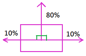
The stochastic environment of grid world with the same setting and the action has the stochastic outcomes, where $80\%$ is the probability we can get our action of our command done, otherwise, we get left or right.
At this time, we are not forgetting the issue of costs, we denote costs as the award function over all possible states, below design might be an incentive to shorten the action sequence, the agent should complete as soon as possible, or the value function of each iterated state might be decreased:
\(R(S)=\left\{\begin{array}{c}+100,for\;M_{1,4}\\-100,for\;M_{2,4}\\-3,othewise\end{array}\right.\)
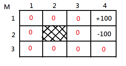
Assume that the initial values are all $0$, except for $M_{1,4}=+100$, $M_{2,4}=-100$ and $\gamma=1$ for simplicity.

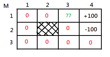
[1]Let’s try to calculate the value of $M_{1,3}$ after a single backup.
➀$V(M_{1,3},E)=-3+0.8\cdot100+0.1\cdot0+0.1\cdot0=77$, for we choose east, the immediate reward of leaving $M_{1,3}$ is $-3$, and $80\%$ chance to arrive $M_{1,4}$ of reward $+100$, $10\%$ chance to bounce back to $M_{1,3}$ of reward $0$, $10\%$ chance to down to $M_{2,3}$ of reward $0$.
➁$V(M_{1,3},W)=-3+0.8\cdot0+0.1\cdot0+0.1\cdot0=-3$, for we choose west, the immediate reward of leaving $M_{1,3}$ is $-3$, and $80\%$ chance to arrive $M_{1,2}$ of reward $0$, $10\%$ chance to bounce back to $M_{1,3}$ of reward $0$, $10\%$ chance to down to $M_{2,3}$ of reward $0$.
➂$V(M_{1,3},N)=-3+0.8\cdot0+0.1\cdot0+0.1\cdot100=7$, for we choose north, the immediate reward of leaving $M_{1,3}$ is $-3$, and $80\%$ chance to bounce back to $M_{1,3}$ of reward $0$, $10\%$ chance to $M_{1,2}$ of reward $0$, $10\%$ chance to $M_{1,4}$ of reward $100$.
➃$V(M_{1,3},S)=-3+0.8\cdot0+0.1\cdot0+0.1\cdot100=7$, for we choose south, the immediate reward of leaving $M_{1,3}$ is $-3$, and $80\%$ go to $M_{2,3}$ of reward $0$, $10\%$ chance to $M_{1,2}$ of reward $0$, $10\%$ chance to $M_{1,4}$ of reward $100$.
Trivially, we have $V(M_{1,3},E)=77$ the maximized value, and the east is the optimal action.

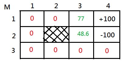
[2]Suppose we are inheriting from above state, where $V(M_{1,3})=77$, what is the value of $M_{2,3}$ after still another single backup?
➀$V(M_{2,3},E)=-3+0.8\cdot-100+0.1\cdot77+0.1\cdot0=-75.3$, for we choose east, the immediate reward of leaving $M_{2,3}$ is $-3$, and $80\%$ chance to arrive $M_{2,4}$ of reward $-100$, $10\%$ chance to $M_{1,3}$ of reward $77$, $10\%$ chance to down to $M_{3,3}$ of reward $0$.
➁$V(M_{2,3},W)=-3+0.8\cdot0+0.1\cdot77+0.1\cdot0=4.7$, for we choose west, the immediate reward of leaving $M_{2,3}$ is $-3$, and $80\%$ chance to bounce back to $M_{2,3}$ of reward $0$, $10\%$ chance to $M_{1,3}$ of reward $77$, $10\%$ chance to down to $M_{3,3}$ of reward $0$.
➂$V(M_{2,3},N)=-3+0.8\cdot77+0.1\cdot0+0.1\cdot-100=48.6$, for we choose north, the immediate reward of leaving $M_{2,3}$ is $-3$, and $80\%$ chance to arrive $M_{1,3}$ of reward $77$, $10\%$ chance to bounce back to $M_{2,3}$ of reward $0$, $10\%$ chance to down to $M_{2,4}$ of reward $-100$.
➃$V(M_{2,3},S)=-3+0.8\cdot0+0.1\cdot0+0.1\cdot-100=-13$, for we choose south, the immediate reward of leaving $M_{2,3}$ is $-3$, and $80\%$ chance to arrive $M_{3,3}$ of reward $0$, $10\%$ chance to bounce back to $M_{2,3}$ of reward $0$, $10\%$ chance to down to $M_{2,4}$ of reward $-100$.
Trivially, we have $V(M_{2,3},N)=48.6$ the maximized value, and the north is the optimal action. Please be recalled that hitting the wall is not the most optimal action any more, it is a major different from prior illustration! That's because we have successfully backup a optimal value of $M_{1,3}=77$.

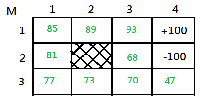
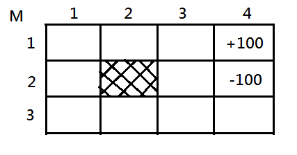
We can propagate value backwards in reverse order of action, executing from $M_{1,4}=+100$, through this grid world and fill every every single state with a better value estimation. If we do this, run the value iteration through convergence, then, we get the following value function:

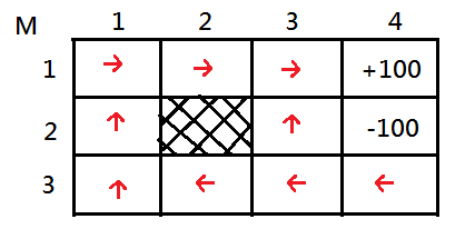
Below is the corresponding mapping of optimal policy containing an optimal action to each distinct state that can maximize its future value function:

After following up above iteration, you might be impressed with such backup process by propagating value function in reverse order sequence of action executing from the goal state back to its previous state.
Value Iteration Under Stochastic Environment Of Two States World
Next, I am going to illustrate in a more general case of stochastic environment containing only 2 states. That’s for the better understanding and ease of computation. In this example, the goal state would be the estimated out target.
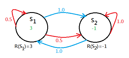
Suppose you are given below 2 states environment with each initialized with value function $0$, the red curve is the action you try to stay in the same state, that says you try to stop, while the blue curve is the action to move to another state:

➀the $S_1$ has both stop and move actions, the stop execution will have $50\%$ chance to stay, $50\%$ chance to move to $S_2$, the move action will have $100\%$ chance to reach $S_2$.
➁the $S_2$ has both stop and move actions, the stop execution will have $100\%$ chance to stay, the move action will have $100\%$ chance to reach $S_1$.
➂the immediate rewards are $R(S_1)=3$ and $R(S_2)=-1$.
Where the move action always succeeding in switching in between the 2 states, the stop action fully works only when it reaches the bad state, $R(S)=-1$. Given $\gamma=0.5$ for a little tricky.
Here is an extra rule, when you apply value iteration, it is in the unit of the whole stochastic environment, not only in some fixed order of state. That is to say the whole system of 2 states would be updated with new value function simultaneously, and then you can start again with the new value functions in the 2 states.
[1]Let’s calculate the value function of $S_1$, beginning over here:
➀$V(S_1,stop)=3+0.5\cdot(0.5\cdot0+0.5\cdot0)=3$, the stop action would come out with $50\%$ chance staying in the same place of reward $0$, $50\%$ chance to the $S_2$ of reward $0$.
➁$V(S_1,move)=3+0.5\cdot(1.0\cdot0)=3$, the move action would come out with $100\%$ chance to the $S_2$ of reward $0$.
Trivially, $V(S_1)=3$, the optimal action of $S_1$ could not be tell at this moment, then, figure out the value function of $S_2$:
➂$V(S_2,stop)=-1+0.5\cdot(1.0\cdot0)=-1$, the stop action would come out with $100\%$ chance to stay in $S_2$ of reward $0$.
➃$V(S_2,move)=-1+0.5\cdot(1.0\cdot0)=-1$, the move action would come out with $100\%$ chance to the $S_1$ of reward $0$.
Trivially, $V(S_2)=-1$, the optimal action of $S_2$ could not be tell at this moment, either.

[2]The current optimal value functions are $V(S_1)=3$ and $V(S_2)=-1$, continue to do the value iteration again:
➀$V(S_1,stop)=3+0.5\cdot(0.5\cdot3+0.5\cdot-1)=3.5$, the stop action would come out with $50\%$ chance staying in the same place of reward $3$, $50\%$ chance to the $S_2$ of reward $-1$.
➁$V(S_1,move)=3+0.5\cdot(1.0\cdot-1)=2.5$, the move action would come out with $100\%$ chance to the $S_2$ of reward $-1$.
Trivially, $V(S_1)=3.5$, the optimal action of $S_1$ could be stop at this moment, then, figure out the value function of $S_2$:
➂$V(S_2,stop)=-1+0.5\cdot(1.0\cdot-1)=-1.5$, the stop action would come out with $100\%$ chance to stay in $S_2$ of reward $-1$.
➃$V(S_2,move)=-1+0.5\cdot(1.0\cdot3)=0.5$, the move action would come out with $100\%$ chance to the $S_1$ of reward $3$.
Trivially, $V(S_2)=0.5$, the optimal action of $S_2$ could be regarded as move at this moment.

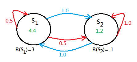
Keep on applying value iteration onto the whole system, we will finally bring the value function of the 2 states to the convergence.

➀$V(S_1,stop)=3+0.5\cdot(0.5\cdot4.4+0.5\cdot1.2)=4.4$, the stop action would come out with $50\%$ chance staying in the same place of reward $4.4$, $50\%$ chance to the $S_2$ of reward $1.2$.
➁$V(S_1,move)=3+0.5\cdot(1.0\cdot1.2)=3.6$, the move action would come out with $100\%$ chance to the $S_2$ of reward $1.2$.
Trivially, $V(S_1)=4.4$, the optimal action of $S_1$ could be stop at this moment, then, figure out the value function of $S_2$:
➂$V(S_2,stop)=-1+0.5\cdot(1.0\cdot1.2)=-0.4$, the stop action would come out with $100\%$ chance to stay in $S_2$ of reward $1.2$.
➃$V(S_2,move)=-1+0.5\cdot(1.0\cdot4.4)=1.2$, the move action would come out with $100\%$ chance to the $S_1$ of reward $4.4$.
Trivially, $V(S_2)=1.2$, the optimal action of $S_2$ could be regarded as move at this moment.
If you treat $S_1$ as sprinting, $S_2$ as jogging, then you will found the most optimal policy for you is to keep on sprinting!! Could we regard it as sprinting costs much fat than jogging, so, everyone should sprint, not jog?
The Optimal Policy Given The Optimal Value Function
At the end of this article, I’d like to generalize the optimal policy. Suppose you have a full understanding of above value iteration process, then, we generalize the optimal policy below:
\(\pi(S)=\underset A{armax}\sum_{S'}P(S'\left|S,A\right.)\cdot V(S')\)
where $\pi(S)$ is the policy $\pi$ for the state $S$, it would yield out the action $A$ that maximizes the value function of a state $S$. The $\gamma$ and the immediate reward has been tossed out, with or without them, th eresult wouldn’t change.
03 Dec 2017
Markov Decision Process In Stochastic Environment
MDP is a prefered framework in stochastic environment and we believe it is full observable. Due to the outcome of action execution is uncertain and random, action choice should not follow conventional planning, instead, an optimal policy.
Self Design Stochastic Environment
The most frequently used example is the information space build on the grid world. This article would just align with world’s grid world for MDP. Alternative illustration of other example would be found in later article in this dev blog.
Let’s begin by a design of 3 by 4 matrix of grid world, $M$. Take $M_{1,4}=+100$, $M_{2,4}=-100$ to be the terminal states with their value specified.

To make it into MDP, we assume actions are somewhar stochastic. Suppose we start from a grid cell and would like to head for the direction we intends to, the deterministic agent will always succeed to move in the direction it plans, on conditions that the target cell on that direction must be available.
But, the action execution result might not go as well as you have expected in the stochastic environment. By our design of stochastic environment, we assume that:
➀only $80\%$ chance for the stochastic agent to move in the direction it expects to.
➁if there is a wall blocking, then, it would bouncce back to the prior starting point, the same cell, with $80\%$ chance.
➂there is a $10\%$ chance to the direction left or right perpendicular to the expected direction, that’s say left or righ of $10\%$ chance respectively.
Above design is just to make the outcome random, that is stochastic.

If the agent at $M_{3,3}$ would like to move to $M_{2,3}$, then, only $80\%$ chance to $M_{2,3}$, $10\%$ chance to $M_{3,2}$, $10\%$ chance to $M_{3,4}$.
If the agent at $M_{3,2}$ would like to move to $M_{2,2}$, then, $80\%$ chance to bounce back to $M_{3,2}$(since $M_{2,2}$ is a blocking wall), $10\%$ chance to $M_{3,1}$, $10\%$ chance to $M_{3,3}$.
Continue fo rthe illustration, if the agent at $M_{1,1}$ would like to move to north(its above), then, it will have totally $90\%$ chance to bounce back to $M_{1,1}$, wherein, $80\%$ chance bounce back from the north(above), $10\%$ chance bounce back from the left, and $10\%$ chance to $M_{1,2}$.
This is a stochastic state transition, so, if you planning a sequence of actions starting from $M_{3,1}$, to reach over the $+100$ at $M_{1,4}$, the final state, you might go N, N, E, E, E. But, with our design, the stochastic agent might move east with $10%$ chance to $M_{3,2}$.
So, we wish to have a planning method that provides an answer no matter where we are, that’s called a policy, where policy assigns actions to any state, that is:
$Poicy\;\pi(S)\rightarrow A$, for each state, we have to regularize a policy, the planning problem now becomes finding the optimal policy.
Conventional Planning In Stochastic Environment Is Insufficient
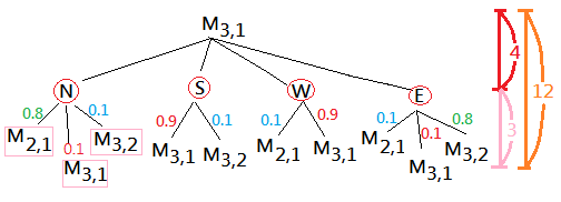
Suppose you are given the information space of the grid world, and would like to start from $M_{3,1}$ to reach the goal state at $M_{1,4}$. By the conventional planning, we might create a tree diagram to construct to possible state transition, since we are now in the stochastic environment, the outcome of action execution to 4 directions, north, south, west, east is not deterministic.

Departuring from $M_{3,1}$, you will have 4 possible action choices, they are N, S, W and E, by our design:
➀if you choose to go north, then, $80\%$ chance to $M_{2,1}$, $10\%$ chance to $M_{3,2}$, $10\%$ chance bounce back to $M_{3,1}$ due to the wall blocking.
➁if you choose to go south, then, $90\%$ chance bounce back to $M_{3,1}$ due to the wall blocking from south of $80\%$ chance and the west of $10\%$ chance, finally, $10\%$ chance to $M_{3,2}$.
➂if you choose to go west, then, $90\%$ chance bounce back to $M_{3,1}$ due to the wall blocking from south of $10\%$ chance and the west of $80\%$ chance, finally, $10\%$ chance to $M_{2,1}$.
➃if you choose to go east, then, $80\%$ chance to $M_{3,2}$, $10\%$ chance to $M_{2,1}$, $10\%$ chance bounce back to $M_{3,1}$.
Take a good look at the tree diagram, the level 1 branching factor is 4, the second level is 3 by grouping the same arriving cell as one variety, then, total branching factor from $M_{3,1}$ would be less than and equal to 12. It would be a large value. If each movement is taken with the cost of 12 branching factors, and many of the next arriving cells has already been visited, conventional planning wouldn't be a good approach, and the whole tree would be too deep.
That's why we need to estimate out a policy to map each state to an optimal action to maximize the value of the state.
Stochastic Environment With Policy By Intuition
We are still using the same information space of the grid world, and the optimal action is the one that provides that you can run around as long as you want. So far, in this example, we are making the test under the assumption that each movement is taken at no cost, which is not the real thing in the real world!!
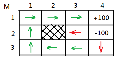
Consider by intuition the optimal action for you to start at below given distinct state(treat each cell to be one state) to end up in the $+100$ state at $M_{1,4}$:
➀begin from $M_{1,1}$, the most optimal step is to move to east of $80\%$ chance to be closed one direct step to $M_{1,4}$.
➁departure from $M_{3,1}$, it would be trivial to move to north, and $80\%$ chance to $M_{2,1}$.
➂kick off at $M_{3,4}$, it has $90\%$ chance to stay in the same place by moving south, since $80\%$ of bouncing back from the south wall, $10\%$ of bouncing back from the east wall. If you choose direct movement to west, then it would come out with $10\%$ danger of falling into the state of $-100$ at $M_{2,4}$. The same $90\%$ chance would get you in $M_{3,4}$, if you choose east movement, cautions must be made that moving to east would get you $10\%$ danger into the state of $-100$ at $M_{2,4}$. Hence, the optimal action is by moving south.
➃take a look at the case when you are beginning from $M_{2,3}$, moving north might not be optimal, you are running the danger of $10\%$ falling into the state of $-100$ at $M_{2,4}$, although, $80\%$ chance to the $M_{1,3}$. If you choose to move south, you still put yourself $10\%$ of the danger to the state of $-100$ at $M_{2,4}$. Why not just hitting the wall by moving west? Choose west movement would get you no any danger of falling to the state of $-100$ at $M_{2,4}$, although $80\%$ bounce back to $M_{2,3}$, you will have $10\%$ chance to the north at $M_{1,3}$ and $10\%$ chance to the south at $M_{3,3}$.

Above graph reveals the possible optimal action for all the states, quiet confusing about hitting wall(this would not be the general case in the real world), and it indeed bring you to the optimal next state. Take $M_{3,4}$ for example, maybe it would contiguous hitting the south wall in the beginning, then turns west sometime later, and behave like W, W, W, N, N, E, E, E to end up.
01 Dec 2017
Markov Decision Process By Intuition
It is the approximation or expression of optimal choice in stochastic environment. Markov Decision Process is an extension of Markov Chain. It takes action control between state transition.
From Markov Chain To Markov Decision Process
Back to have a glance at the Markov Chain, the future state value might be stablized. We wonder about the next state from current state, and would like to estimate it out. The estimation involves one extra consideration of action choice. The regularized solution would be a policy for each state to take its optimal action to maximize its value over horizon of some magnitude.
The Markov Decision Process Components And Features
➀a set of states, denote it as $S$.
➁a set of actions associated with states, denoted as $A$.
➂state transition probability, denote as $P(S_{t+1}\left|S_t\right.,a_t)$; where the Markov property claims:
\(P(S_{t+1}\left|S_t\right.,a_t)=P(S_{t+1}\left|S_t\right.,S_{t-1},\dots,S_0,a_t,a_{t-1},\dots,a_0)\)
That is to say given the current state and action, the next state is independent of the previous states and actions. The current state estimates all that is relevant about the world to predict what the next state will be.
➃immediate reward of each state, denoted as $R(S)$. Some article pertaining to MDP would treat it as the cost, which would also be used in our future illustration.
The above four items are the major components in MDP. And from now on, we would use MDP in this article, even more, the whole dev blog, to stand for the Markov Decision Process.
MDP takes action in decision making process with a hope that it can regularize a policy for each state to have an optimal choice of action to maximize its expected state value estimated over herizon of magnitude of a long term, even infinity.
In advance to involve the policy, it would be better for us to distinguish in between conventional planning and MDP policy.
Conventional Plan v.s. MDP Policy
➀a plan is either an ordered list of actions or a partially ordered set of actions, executed without reference to the state of the environment.
➁for conditional planing, we treat it to act differently depending on the observation about the state of the world.
➂in MDP, it is typically to compute a whole policy rather than a simple plan.
A policy is a mapping from states to actions, whatever state you happen to start from, a policy is the best to apply now.
Stochastic v.s. Deterministic
You still ponder why to replace conventional planning with MDP policy, in this paragraph, we will further investigate in the differences in between stochastic and deterministic.
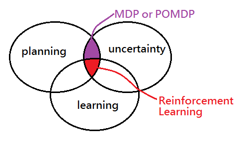
Below shows you an image of the appropriate discipline with respect to the desired behavior under the environment condition. For planning under uncertainty, we intend to refer to MDP or POMDP(PO means partial observable, would be discussed in another article), for learning, planning under under uncertainty, we will step into the reinforcement learning, still in another article.

Next to make a unique identity of stochastic and determninistic.
➀stochastic is an environment where the outcome of an action is somewhat random, that means, the execution result might not go as well as you have expected.
➁determninistic is an environment where the outcome of an action is predictable and always the same, that means the execution result would go as well as you have expected.

For the discipline of MDP, we are full observable under stochastic environment. Actually, full observable is impossible, we just believe that the design or hypothesis on the experimental environment is under the full control, but, anything out of the imagination would just errupt. More precisely, we should treat almost every issue under partial observable, and it would be the domain of POMDP(Partial Observable Markov Decision Process), discussed in another article in my dev blog. At this moment, focus on MDP only and hypnotize ourself that we have control everything.
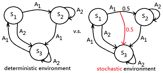
At the end of this section, I would like to get you a clear expression of stochastic versus deterministic. Given below diagram of three states, with each state has two actions. The left side reveals the deterministic environment, each action is taken from each state to its next state, and the execution result is the same as expected; whereas the right side exhibits the stochastic environment, the execution of action $A_1$ from state $S_1$ has been branched into two results by random with each has $0.5$ chance to reach next state $S_2$ and $S_3$ respectively. This illustrates the result of action execution in stochastic environment is random.

01 Dec 2017
Markov Chain
It is the approximation or expression of stochastic environment. Markov Chain also known by Markov Process. Cautions must be made that it is not equivalent to the Markov Decision Process, because it has no action control.
A Glance At The Markov Chain
The Markov Chain consists of finite number of discrete states, probabilistic transition between states, maybe rewards of each state, and the most important is Markov Chain has no action control. No action to take, just from one state to another state.

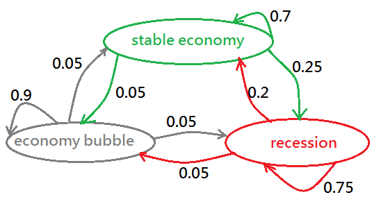
The 3 ellipses in different colors are individual states, where the green color indicates the stable state, the gray color stands for bubble state, the red color means the recession state. The transition probability is along each curve with its direction by the arrow.
You can see that no any reward found in above graph, since the Markov Process don't always has the reward values associated with them.
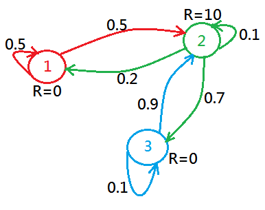
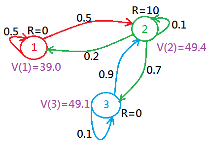
Still another example of Markov Process is exhibited below, in this example, we add immediate reward on each state, R=0 for state 1, R=10 for state 2, R=0 for state 3:

Notes that:
➀the probability on all the outgoing arcs of each state sum to one!
➁the Markov Process could be constructed with or without the reward in each state, it depends on artificial design.
➂no action to take, just transite from one state to another state.
The Markov Chain Components And Features
The primary components of the Markov Chain:
➀states
➁transition probabilities
➂rewards
The major feature is that it has no actions to take, no decisions to make, just transits in between states.
The Markov Property
In Markov Process, next state is determined only by the current state, which is the Markov property.
Value Of A State
In this article, we express the value of a state over an infinite expected discounted horizon, and denote as V(S). That is to say we define the inifnite expected discounted reward as a function of the starting state. We’ll abbreviate V(S) as the value of a state.
Here comes the question, how much total reward do we expect to get if we start in state S?
➀we will get an immediate reward R(S), just right in state S.
➁we will then get some reward in the future. The reward we get in the future is not worth as much to us as reward in the present, so we multiply by a discount factor gamma $\gamma$.
\(V(S)=R(S)+\gamma\cdot(?)\)
What The Future Might Be?
Given a intuition of value state, and a possible roadmap, what is the future value in the long run? The expected long term value of the next state is by summing over all possible next states, $S’$;where $S’$ is the product of:
➀the probability of making transition from $S$ to $S’$, $P(S'\left|S\right.)$.
➁the infinite horizon expected discounted reward(or the value of S’), $V(S')$.
At this moment, take the future value of current state $S$ as immediate reward of current valus $S$ plus the expected long term value of the next state $S’$:
\(V(S)=R(S)+\gamma\cdot\sum_{S'}P(S'\left|S\right.)\cdot V(S')\)
Suppose we know $R$ and $P$, next to compute $V$, if $n$ is the number of states in the domain, then, we have a set of $n$ equations in $n$ unknowns(the value of each state).
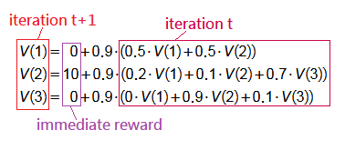
Continue with the three states example, given $\gamma=0.9$, by using above equation of intuition could we have future value illustration in below, whereas, in this example the initial value of each state is unknown:

If $\gamma=0$, then, the $V(S)$ of each state would just be the same as their immediate reward.
If $\gamma$ is small, but non-zero, then the value would be smaller.
Suppose after summing the next states $S’$ over a long horizon, we finally get it to the stable state with each state has its stable value.

What’s The Optimal Choice?
Here we are against a problem, if you are in one of the three states, what would be the optimal choice to get you the best next state? If such answer exists, it involves deterministics from within stochastic environment due to probabilistic state transition as a result of random action result. We’d like to further migrate into the field of Markov Decision Process, the computation requires extra deterministics.
