05 Mar 2019
Prologue To The Bellman Operator Makes Convergence
By contiguous Bellman update, the value of each state eventually get converged, this happens a lot in reinforcement learning.
Begin By Bellman Operator - B
[1]
Beginning
Let B be an operator, or mapping from value function to value function. You give a Q function, the Bellman operator will give you back, possibly, a different Q function. You can treat B a function from Q functions to Q functions.
[2]
Definition of Bellman operator
$BQ$=$R(S,A)$+$\gamma\cdot{\textstyle\sum_{S’}}P(S’\vert S,A)\cdot max_{A’}Q(S’,A’)$
Give B a Q function, the new thing we get out when we apply B onto Q, has the property that at the state action pair $(S,A)$, it is equal to the immediate reward plus the discounted expected value of the next state, $S'$.
So, Q goes in, BQ goes out, treat BQ a new function.
[3]
Another way of writing
With Bellman operator - B, we can have below alternatives:
➀$Q^{\ast}$=$BQ^{\ast}$ is another way of writing Bellman equation.
➁$Q_{t}$=$BQ_{t-1}$ is another way of writing value iteration.
Contraction Mapping
[1]
Definition
It happens a lot in reinforcement learning. Take B to be an operator,
$\;\;$if for all $F$,$G$ and some $0\leq\gamma<1$,
$\;\;\vert\vert BF-BG\vert\vert_{\infty}\leq\gamma\cdot \vert\vert F-G\vert\vert_{\infty}$,
then B is contraction mapping, where
➀$F$ and $G$ are value functions of Q form.
➁$\vert\vert Q\vert\vert_{\infty}$=$max_{S,A}\vert Q(S,A)\vert$, this notation sometimes called the infinity form, the max norm.
➂$\vert\vert F-G\vert\vert_{\infty}$ this means the biggest difference between $F$ and $G$.
The contraction mapping means whatever largest difference is, we are going to multiply it by something that makes it even smaller. If you apply B onto $F$ and $G$, the distance between the resulting function is even closer together than they started.
[2]
Hints
It’s the case that over time as we apply the Bellman operator - B over and over again, the state action pair where their maximum is, might change every time.
➀$\vert\vert F-G\vert\vert_{\infty}$, this maximum norm is computing for the specific value function of $F$ and $G$, where their absolute difference is given the biggest.
➁$\vert\vert BF-BG\vert\vert_{\infty}$ is different from $\vert\vert F-G\vert\vert_{\infty}$ in that there is no reason that $\vert\vert BF-BG\vert\vert_{\infty}$ needs to the the same over and over again.
[3]
Properties
If B is an operaton leads to contraction mapping:
➀$F^{\ast}$=$BF^{\ast}$ has a unique solution.
proof:
Suppose we have $F_{1}^{\ast}$=$BF^{\ast}$ and $F_{1}^{\ast}$=$BF^{\ast}$, then $F^{\ast}$=$F_{1}^{\ast}$=$F_{2}^{\ast}$ just holds to hvave the unique $F^{\ast}$.
➁$F_{t}$=$BF_{t-1}$, this leads to $F_{t}\rightarrow F^{\ast}$, value iteration converges.
proof::mjtsai1974
Start from definition, we have:
$\vert\vert BF_{t-1}-BF^{\ast}\vert\vert_{\infty}\leq\gamma\cdot \vert\vert F_{t-1}-F^{\ast}\vert\vert_{\infty}$…[A]
$\Rightarrow \vert\vert F_{t}-F^{\ast}\vert\vert_{\infty}\leq\gamma\cdot \vert\vert F_{t-1}-F^{\ast}\vert\vert_{\infty}$
By mathematics induction, below deduction holds:
$\vert\vert BF_{t}-BF^{\ast}\vert\vert_{\infty}\leq\gamma\cdot \vert\vert F_{t}-F^{\ast}\vert\vert_{\infty}\leq\gamma^{2}\cdot \vert\vert F_{t-1}-F^{\ast}\vert\vert_{\infty}$…[B]
Next, substract [B] from [A], we get:
$\vert\vert BF_{t-1}-BF_{t}\vert\vert_{\infty}\leq\gamma\cdot(1-\gamma)\cdot\vert\vert F_{t-1}-F^{\ast}\vert\vert_{\infty}$
$\Rightarrow\vert\vert BF_{t-1}-BF_{t+1}\vert\vert_{\infty}\leq\gamma\cdot(1-\gamma^{2})\cdot\vert\vert F_{t-1}-F^{\ast}\vert\vert_{\infty}$
$\Rightarrow\vert\vert BF_{t-1}-BF_{t+2}\vert\vert_{\infty}\leq\gamma\cdot(1-\gamma^{3})\cdot\vert\vert F_{t-1}-F^{\ast}\vert\vert_{\infty}$
…
$\Rightarrow\vert\vert BF_{t-1}-BF_{t+n}\vert\vert_{\infty}\leq\gamma\cdot(1-\gamma^{n+1})\cdot\vert\vert F_{t-1}-F^{\ast}\vert\vert_{\infty}$
We can tell that the first difference term will become stable with respect to each transition in $t$, $t+1$,…, the vaule of $F$ just converges to $F^{\ast}$. As $n\rightarrow\infty$, we have $\gamma\cdot(1-\gamma^{n})\rightarrow \gamma$, for $\gamma<1$just holds.
If $F$ is evaluated from $t-1$, after $n\rightarrow\infty$, it will just converge to $F^{\ast}$ with the acceptable difference no more than $\gamma$ times the difference between the original departuring $F_{t-1}$ and the final expected $F^{\ast}$.
The Bellman Operator Contracts: The Proof
Given $Q_{1}$ and $Q_{2}$, then $\vert\vert BQ_1-BQ_2\vert\vert_\infty\leq\gamma\cdot\vert\vert Q_1-Q_2\vert\vert_\infty$, this says that after we apply B onto $Q_{1}$ and $Q_{2}$, the distance between them is less than or equal to $\gamma$ times the original difference betwen them before we apply it.
So, by applying the Bellman operator, we move these 2 $Q$ functions closer together.
In this section, we are going to prove the definition of contraction mapping by B.
proof:
➀when we apply B onto $Q$:
$\lbrack BQ\rbrack(S,A)$=$R(SA)$+$\gamma\cdot\sum_{S’}P(S’\vert S,A)\cdot max_{A’}Q(S’,A’)$
➁the next thing is to unpack the definition of the max norm.
$\vert\vert BQ_{1}-BQ_{2}\vert\vert_{\infty}$
=$max_{S,A}\vert BQ_{1}(S,A)-BQ_{2}(S,A)\vert$
…we are going to maximize over all state action pair
=$max_{S,A}\vert R(S,A)+\gamma\cdot\sum_{S’}P(S’\vert S,A)\cdot max_{A_{Q_{1}}’}Q_{1}(S’,A_{Q_{1}}’)$
$\;\;$-$R(S,A)-\gamma\cdot\sum_{S’}P(S’\vert S,A)\cdot max_{A_{Q_{2}}’}Q_{2}(S’,A_{Q_{2}}’)\vert$
=$max_{S,A}\vert \gamma\cdot\sum_{S’}P(S’\vert S,A)\cdot max_{A_{Q_{1}}’}Q_{1}(S’,A_{Q_{1}}’)$
$\;\;$-$\gamma\cdot\sum_{S’}P(S’\vert S,A)\cdot max_{A_{Q_{2}}’}Q_{2}(S’,A_{Q_{2}}’)\vert$
=$max_{S,A}\gamma\cdot\sum_{S’}P(S’\vert S,A)\cdot\vert max_{A_{Q_{1}}’}Q_{1}(S’,A_{Q_{1}}’)$
$\;\;$-$max_{A_{Q_{2}}’}Q_{2}(S’,A_{Q_{2}}’)\vert$
$\leq \gamma\cdot max_{S’}\vert max_{A_{Q_{1}}’}Q_{1}(S’,A_{Q_{1}}’)$
$\;\;$-$max_{A_{Q_{2}}’}Q_{2}(S’,A_{Q_{2}}’)\vert$
=$\gamma\cdot max_{S’,A_{Q_{1}}’,A_{Q_{2}}’}\vert Q_{1}(S’,A_{Q_{1}}’)$-$Q_{2}(S’,A_{Q_{2}}’)\vert$
By tossing out the weight combination, the term $\sum_{S'}P(S'\vert S,A)$ of $Q$ values, we just worry about the $S'$, where the difference is the largest, the weighted average or the convex combination could not be larger than the biggest difference at any $S'$, therefore, no need to keep $max_{S,A}$.
➂$\vert\vert BQ_1-BQ_2\vert\vert_\infty\leq\gamma\cdot\vert\vert Q_1-Q_2\vert\vert_\infty$ is thus proved.
Maximum Is Non-Expansion
For all $f$ and $g$, we have:
$\vert max_{a}f(a)-max_{a}g(a)\vert\leq max_{a}\vert f(a)-g(a)\vert$
proof:
$\Rightarrow$Suppose we have below maximum argument holds:
➀$maxarg_{a}f(a)$=$a_{1}$
➁$maxarg_{a}g(a)$=$a_{2}$
And, we assume $f(a_{1})\geq g(a_{2})$, this assumption owuld not lose generality in this proof, we can also prove with the assumption $f(a_{1})\leq g(a_{2})$.
$\Rightarrow$since $maxarg_{a}g(a)$=$a_{2}$, we have $g(a_{2})\geq g(a_{1})$
$\Rightarrow\vert max_{a}f(a)-max_{a}g(a)\vert$
=$f(a_{1})-g(a_{2})$
$\leq f(a_{1})-g(a_{1})$
=$max_{a}\vert f(a)-g(a)\vert$
Addendum
➀Temporal Difference Convergence, Charles IsBell, Michael Littman, Reinforcement Learning By Georgia Tech(CS8803)
➁An introduction to Q-Learning: reinforcement learning, ADL
19 Feb 2019
Not just learn the value, TD(Temporal Difference) rule with action control in Q form would learn the values of different actions we might take as a way to figure out the most optimal(maximum valued) behavior in each state.
By given enough data, enough time, TD with action control would just do the right thing and eventually converge.
Glance At The Q-Learning
[1]
Overview
Here I am just to have a simplistic overview of Q-learning:
➀Q-learning is a value-based reinforcement learning algorithm, which is used to find the most optimal(best) policy to choose the action that can maximize the value of each state by using a Q function.
➁the Q function takes state and action as input parameters.
$Q^{\pi}(S_{t},A_{t})$=$E\lbrack R_{t+1}+\gamma\cdot R_{t+2}+\gamma^{2}\cdot R_{t+3}+…\vert S_{t},A_{t}\rbrack$
The $\pi$ indicates the $Q$ function asks for policy could be expressed in the form of expected discounted cumulative reward, given $S_{t}$ and $A_{t}$.
➂take action $A$ to transite from state $S$ to $S’$
$Q_{T}(S,A)$
=$Q_{T-1}(S,A)$+$\alpha_{T}\cdot(R(S,A)$+$\gamma\cdot max_{A’}Q_{T-1}(S’,A’)$-$Q_{T-1}(S,A))$…[A]
By repeating above Bellman equation in Q form, the Q value will finally get converged, usually denoted as $Q^{*}(S,A)$, and it’s the policy for you to take action $A$ when you are in state $S$ to get the maximum value.
[2]
Notes::mjtsai1974
As to equation [A], it could be further expanded:
$Q_{T}(S,A)$
=$Q_{T-1}(S,A)$+$\alpha_{T}\cdot(R(S,A)$+$\gamma\cdot max_{A’}Q_{T-1}(S’,A’)$-$Q_{T-1}(S,A))$…[A]
=$Q_{T-1}(S,A)$+$\alpha_{T}\cdot(R(S,A)$+$\gamma\cdot (\sum_{S’}P(S’\vert S,A)\cdot max_{A’}Q_{T-1}(S’,A’))$-$Q_{T-1}(S,A))$…[B]
Say it [B], where the term $(\sum_{S’}P(S’\vert S,A)\cdot max_{A’}Q_{T-1}(S’,A’))$ in [B] could be treated as $max_{A’}Q_{T-1}(S’,A’)$ in [A].
➀if we know the probability transition from $S$ to $S’$, its associated immediate reward, we can take advantage of [B].
➁if we neither know probability distribution of state $S$, nor the immediate reward, we can just use [A], take only the Q value learned in last eposide.
See, the Q form is just expressed in terms of temporal difference.
The Q form is quiet usefule in the reinforcement learning, when we are under the condition that we know nothing about the immediate reward and the probability distribution from current state to next state is uncertain, it is converinet to use this Q value as the experience.
Bellman Equation: With versus Without Actions
[1]
Without actions
➀no action in value function:
$V(S)$=$R(S)$+$\gamma\cdot\sum_{S’}P(S’\vert S, A)\cdot V(S’)$
The value function $V(S)$ of state $S$ takes no action control into consideration, the term $P(S’\vert S, A)$ indicates the we are in stochastic MDP model, the outcome of action execution is uncertain.
➁$TD(0)$ isomorphism:
$V_{T}(S_{t-1})$=$V_{T}(S_{t-1})$+$\alpha_{T}\cdot (r_{t}+\gamma\cdot V_{T-1}(S_{t})-V_{T-1}(S_{t-1}))$
By using $TD(0)$ to update the value of $S_{t-1}$ when transiting from $S_{t-1}$ to $S_{t}$ in one eposide.
[2]
With actions
➀the Q form value function:
$Q(S,A)$=$R(S,A)$+$\gamma\cdot\sum_{S’}P(S’\vert S, A)\cdot max_{A’}Q(S’,A’)$
The value function now takes action into concern, after transiting from $S$ to $S’$, targeting at the action $A’$ chose by $S’$ to maximize value of $S’$, the term $Q(S’,A’)$.
➁$TD(0)$ isomorphism:
$Q_{T}(S_{t-1},A_{t-1})$=$Q_{T-1}(S_{t-1},A_{t-1})$+$\alpha_{T}\cdot (r_{t}+\gamma\cdot max_{A_{t}}Q_{T-1}(S_{t},A_{t})-Q_{T-1}(S_{t-1},A_{t-1}))$
By using $TD(0)$ to update the value of $S_{t-1}$ in one eposide, be noted the term $max_{A_{t}}Q_{T-1}(S_{t},A_{t})$ aims at the action $A_{t}$ chose by $S_{t}$ that can maximize the value of $S_{t}$, the term $Q_{T-1}(S_{t},A_{t})$. If such $A_t$ exists and can maximize $Q_{T}(S_{t},A_{t})$ across all eposide $T$, then it is just the policy to choose $A_{t}$.
Approximations
[1]
We know the whole MDP model
If we know the whole MDP model, then, synchronuous update, simply by applying Bellman equation:
$Q_{T}(S,A)$=$R(S,A)$+$\gamma\cdot\sum_{S’}P(S’\vert S,A)\cdot max_{A’}Q_{T-1}(S’,A’)$
➀as to the term $R(S,A)$, this is the immediate reward, $A$ is just the best action taken by state $S$ to transite to $S’$. Because the whole MDP model is known, we know this $R(S,A)$.
➁the synchronuous update is by suming over all probabilistic transitions from $S$ to $S’$, given action $A$.
➂we take the old $Q_{T-1}(S’,A’)$ value estimated in eposide $T-1$ and do the Bellman update in specific state, action pair or particular state connection pair.
[2]
the whole MDP model is not clear, but $Q_{T-1}^{\ast}(S_{t-1},A_{t-1})$ is known
When we transite from $S_{t-1}$ by action $A_{t-1}$ to $S_{t}$, if we know $Q_{T-1}^{\ast}(S_{t},A_{t})$, we could use it to learn $Q_{T}^{*}(S_{t-1},A_{t-1})$ by sampling asynchronuously update.
$Q_{T}(S_{t-1},A_{t-1})$=$Q_{T-1}(S_{t-1},A_{t-1})$+$\alpha_{T}\cdot(r_{t}+\gamma\cdot max_{A_{t}}Q_{T-1}^{\ast}(S_{t},A_{t})-Q_{T-1}(S_{t-1},A_{t-1}))$
Where we can take $Q^{\ast}(S_{t-1},A_{t-1})$=$Q_{T}(S_{t-1},A_{t-1})$, the $Q_{T}(S_{t-1},A_{t-1})$ learned would eventually converge to $Q^{\ast}(S_{t-1},A_{t-1})$.
[3]
Inspiration::mjtsai1974
The $Q^{\ast}$ value of $(S,A)$could be estimated from given data, suppose we are evaluating $Q^{\ast}(S_{t-1},A_{t-1})$, here are the point and concern:
➀should we estimate $Q^{\ast}(S_{t-1},A_{t-1})$ base on the whole given data and use it for $Q_{t}^{\ast}(S_{t-1},A_{t-1})$, where $t\in all\;T$? Or,
➁should we estimate $Q_{T-1}^{\ast}(S_{t-1},A_{t-1})$ on sample from eposide $1$ to $T-1$, when we are now evaluating in eposide $T$, the $T$-th eposide?
➂if we choose ➀, would we just ignore the partial observe mechanism in this learning process? Or,
➃first learn by ➀, then we just learn by ➁, after the end is reached, we do the estimate for each distinct $Q(S,A)$ pair, repeat each iteration of learning in ➁ with respect to each $Q(S,A)$ in each eposide of transition from $S_{t-1}$ to $S_{t}$, finally do the adjustment in each learning eposide in ➁, by adjust learning rate or discount factor!!!
➄succeed to ➃, compare with the learning result in ➀, until the norm of the difference has been brought to the minimum, if we treat the learning result in ➀ and ➁ as vectors.
By this scenario of learning by ➀ then by ➁ to get the learning rate and discounted factor converged, we assume the current given data is the complete data set for the complete MDP model we know, so far; and the very next time, something unobservable in last session has been observed in this session, just triggers the whole learning process again in the very next session!!!
Addendum
➀Temporal Difference Convergence, Charles IsBell, Michael Littman, Reinforcement Learning By Georgia Tech(CS8803)
➁An introduction to Q-Learning: reinforcement learning, ADL
22 Jan 2019
Prologue To The Temporal Difference Learning - Part 2
This is the part 2, new introduce $TD(0)$, continue with advantages and cons of $TD(0)$, $TD(1)$, come out with conclusion in TD($\lambda$).
$TD(0)$ Algorithm: $\lambda$=$0$
This is by taking $\lambda$=$0$ in $TD(\lambda)$ algorithm.
[The rule]
Eposide $T$:
$\;\;$For all $S$, $e(S)$=$0$ at start of eposide, $V_{T}(S)$=$V_{T-1}(S)$
$\;\;$After $S_{t-1}\xrightarrow{r_{t}}S_{t}$:(from step $t-1$ to $t$ with reward $r_{t}$)
$\;\;\;e(S_{t-1})$=$e(S_{t-1})$+$1$:
$\;\;\;\;$Update eligibility of $S_{t-1}$ after arriving to $S_{t}$
$\;\;$For all $S$,
$\;\;V_{T}(S)$=$V_{T-1}(S)$+$\alpha_{T}\cdot(r_{t}+\gamma\cdot V_{T-1}(S_{t})-V_{T-1}(S_{t-1}))$…[A]
$\;\;\;e(S_{t-1})$=$0\cdot\gamma\cdot e(S_{t-1})$=$0$:
$\;\;\;\;$before transite from $S_{t-1}$ to $S_{t}$ in next iteration, we can easily tell that the eligibility of state $S$ is always zero.
[Notes]
➀the 2nd part of (A) is sum of the reward plus the the discounted value of the state we just arrived, minus the state value we just left; where these state values are all evaluated in last iteration. It could just be the temporal difference.
➁we are going to apply the temporal difference onto $S$ itself only, with no proportion to the eligibility of any other states, and the learning rate would be specified for we don’t want it to move too much.
➂after the state has been iterated, decay or decrease its eligibility with $\lambda\cdot\gamma$, in their given value, in $TD(0)$, $\lambda$=$0$, the eligibility of state $S$ is always zero.
➃and we are backing up to next stae.
[Caution]
➀all the $S$ are all being done in similar approach.
➁the value at state $S$(the $S$ in [A]) is going to be updated on this quantity, $r_{t}+\gamma\cdot V_{T-1}(S_{t})-V_{T-1}(S_{t-1})$, which is the same for everybody, doesn't depend on which $S$ we are updating, and $e(S)$=$1$ is specific to the state $S$ at the moment we are evaluating(looking at).
MLE(Maximum Likelihood Estimate) And $TD(0)$ Algorithm
[1]
MLE
Given data of a lot trajectories and we are under the condition that we are in $S_{t-1}$, and we don’t know what state we are going to end up in. But, there exists some probability of $r_{t}$+$\gamma\cdot V_{T-1}(S_{t})$-$V_{T-1}(S_{t-1})$.
If we take expectation of [A], then:
$V_{T}(S_{t-1})$=$E_{S_{t}}[r_{t}+\gamma\cdot V_{T-1}(S_{t})]$…[B]
We could treat it as the MLE of $V_{T}(S_{t-1})$ over all possible $V_{T-1}(S_{t})$. What we are doing is just sampling different possible $S_{t}$ values, that is $V_{T-1}(S_{t})$, and is crossing over different trajectories for we have dataset of trajectories.
We are just taking an expectation over what we get as the next state of the reward plus the discounted estimated value(evaluated in last eposide) of that next state.
[2]
Why [B] is supposed to be the MLE?
$\;\;$[B] is the MLE
proof::mjtsai1974
➀$V_{T}(S_{t-1})$
=$V_{T-1}(S_{t-1})$+$\alpha_{T}\cdot(r_{t}+\gamma\cdot V_{T-1}(S_{t})-V_{T-1}(S_{t-1}))$
=$V_{T-1}(S_{t-1})\cdot(1-\alpha_{T})$+$\alpha_{T}\cdot(r_{t}+\gamma\cdot V_{T-1}(S_{t}))$…[B.1]
This is the value of $S_{t-1}$ in eposide $T$, when transiting from $S_{t-1}$ to $S_{t}$, and remind that we are given data of a lot trajectories with each containing state transition in it.
➁suppose we are in $S_{t-1}$ in one trajectory, and the next $S_{t}$ does exist, there exists $k$ such $S_{t}$ and $n-k$ different states of $S_{t}$, and totally $n$ trajectories in the given data. Therefore, there exists some probability $P(S_{t}\vert S_{t-1})$=$\frac {k}{n}$.
➂$V_{T}(S_{t-1})$
=$\sum_{S{t}}P(S_{t}\vert S_{t-1})\cdot([B.1])$
=$E_{S_{t}}[r_{t}+\gamma\cdot V_{T-1}(S_{t})]$ just holds.
, where $V_{T-1}(S_{t-1})\cdot(1-\alpha_{T})$ and $\alpha_{T}\cdot(r_{t}+\gamma\cdot V_{T-1}(S_{t}))$ are some values varying in each trajectory, the former is the departuring state, the later is the ending state, $\alpha_{T}$ is the learning rate, depends on how you would like the learning process to be. I just use the term $r_{t}+\gamma\cdot V_{T-1}(S_{t})$ to be the random variable to be taken expectation.
Illustration: The Idea Of TD(0) After TD(1)
[1]
The given example
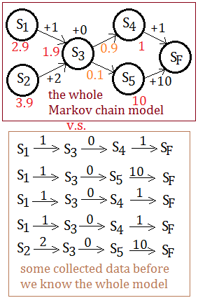
Succeeding to the same example as part 1 article, this time we are given data of 5 trajectories, the red quantity is the value of the state after backup propagation with $\gamma$=$1$. Recall that each distinct state’s initial value is $0$. We’d like to ask for the value of $S_{2}$ in the 5-th eposide.
[2]
By using TD(1)
➀we can deduce it out the temporal difference term:
$\triangle V_{T}(S_{2})$
=$r_{2}$+$\gamma\cdot r_{3}$+$\gamma^{2}\cdot r_{5}$+$\gamma^{3}\cdot V_{T-1}(S_{F})-V_{T-1}(S_{2})$
=$12$
➁$V_{T}(S_{2})$
=$V_{T-1}(S_{2})$+$\triangle V_{T}(S_{2})$
=$0$+$12$
=$12$
[3]
By using MLE
$V_{T}(S_{2})$
=$r_{2}$+$\gamma\cdot P(S_{3}\vert S_{2})\cdot V_{T}(S_{3})$
=$r_{2}$+$\gamma\cdot P(S_{3}\vert S_{2})\cdot [r_{3}$
$\;\;$+$\gamma\cdot (P(S_{4}\vert S_{3})\cdot(V_{T}(S_{4}))$
$\;\;\;\;$+$P(S_{5}\vert S_{3})\cdot (V_{T}(S_{5}))]$
=$r_{2}$+$\gamma\cdot P(S_{3}\vert S_{2})\cdot [r_{3}$
$\;\;$+$\gamma\cdot (P(S_{4}\vert S_{3})\cdot(r_{4}+\gamma\cdot P(S_{F}\vert S_{4})\cdot V_{T}(S_{F}))$
$\;\;\;\;$+$P(S_{5}\vert S_{3})\cdot (r_{5}+\gamma\cdot P(S_{F}\vert S_{5})\cdot V_{T}(S_{F})))]$
, and from data, we have probability of transition that
➀$\gamma$=$1$
➁$P(S_{3}\vert S_{2})$=$1$
➂$P(S_{4}\vert S_{3})$=$0.6$
➃$P(S_{5}\vert S_{3})$=$0.4$
➄$P(S_{F}\vert S_{4})$=$1$
➅$P(S_{F}\vert S_{5})$=$1$
Therefore,
$V_{T}(S_{2})$
=$2$+$1\cdot 1\cdot [0$
$\;\;$+$1\cdot (0.6\cdot(1+1\cdot 1\cdot 0)$
$\;\;\;\;$+$0.4\cdot (10+1\cdot 1\cdot 0))]$
=$6.6$, by the same approach, $V_{T}(S_{1})$=$5.6$.
Cautions must be made that by using MLE for $V_{T}(S_{2})$, we choose to refer to the same eposide $T$, not $T-1$, why?
This is all due to we are doing the estimiation by using data.
[4]
The breakdown
Please recall in Temporal Difference Learning - Part 1, I have figured out that $V_{T}(S_{1})$=$2.9$, $V_{T}(S_{2})$=$3.9$, $V_{T}(S_{3})$=$1.9$, by using both backup propagation and expect discounted reward in the section of ReCap The Backup In Markov Chain.
The MLE of $V_{T}(S_{2})$=$6.6$, which is more, whereas the $TD(1)$ estimate is $12$, a lot more, all wrong, except for $V_{T}(S_{2})$=$3.9$ by using backup based on the whole model. Why MLE is less wrong? Why $TD(1)$ estimate is so far off?
➀when we compute the $TD(1)$ estimate, we use only the 5-th trajectory, one of the five trajectories to propagate the information back.
➁when we use MLE for the estimation, we use all data, more information, more accurate. The more might not be the better, but, we can resort the inaccuracy of MLE of $V_{T}(S_{2})$=$6.6$ to that we don't have the complete data set to build this whole MC model.
Specifically be noted that $TD(1)$ is alos be treated as outcome-based estimate for it uses the immedaite reward and ignores the intermediate encountered states' value.
[5]
A tiny finding
We have a tiny finding that $TD(0)$ relates current state's value to next most closed state's value, is more like MLE estimate, even if we are using it in one trajectory, the 5-th in this illustration.
The temporal difference is about to learn to make prediction of states value for these states transit over time in the unit of one distinct trajectory, whereas the MLE tends to estimate states’ value accrossing all trajectories in given sample.
The argument in between $TD(0)$, $TD(1)$ and MLE is in that we don't have the full image of the Markov chain model, with only a little sampling data.
[1]
Summary of these equations
I’d like to step further to deeper inside in the concept with $TD(0)$ and $TD(1)$. Given below 3 expression:
➀$V_{T}(S_{t-1})$
=$V_{T-1}(S_{t-1})$+$\alpha_{T}\cdot(r_{t}+\gamma\cdot V_{T-1}(S_{t})-V_{T-1}(S_{t-1}))$…[A]
➁$V_{T}(S_{t-1})$
=$E_{S_{t}}[r_{t}+\gamma\cdot V_{T-1}(S_{t})]$…[B]
➂$V_{T}(S_{t-1})$
=$E[r_{t}+\gamma\cdot r_{t+1}+\gamma^{2}\cdot r_{t+2}+\gamma^{3}\cdot r_{t+3}+…]$…[C]
, where [A] is the regular expression in temporal difference, works for both $TD(0)$ and $TD(1)$, the difference is in $TD(0)$ rule the eligibility of the evaluated state would be reset to $0$; the equation [B] is by taking expect of [A], more description is in $TD(0)$ related section; whereas [C] is the idea by taking only the reward sequence that we saw, ignoring the estimate we might have gotten in some other states, which is the spiritual $TD(1)$.
[2]
Why toss out $\gamma^{k}\cdot V_{T-1}(S_{t+k})-V_{T-1}(S_{t-1})$?
Moreover, the full [C] expression should be refined as:
$V_{T}(S_{t-1})$
=$E[r_{t}+\gamma\cdot r_{t+1}+\gamma^{2}\cdot r_{t+2}$
$\;\;+…+\gamma^{k-1}\cdot r_{t+k-1}+\gamma^{k}\cdot V_{T-1}(S_{t+k})-V_{T-1}(S_{t-1})]$…[D]
The reason we ignore these 2 terms $\gamma^{k}\cdot V_{T-1}(S_{t+k})-V_{T-1}(S_{t-1})$ is that when $k$ is quiet large, the $\gamma^{k}$ would then approach $0$, and $V_{T-1}(S_{t-1})$'s initial value is $0$ in one eposide, if $S_{t-1}$ is the target state to be evaluated, especially the very first time it is evaluated.
[3]
Evaluation on [B] and [C]
By using [C], is just like the $S_{2}$ in the 5-th trajectory in above illustrated example, however, when the trajectory is an infinite series, the $TD(1)$ also does the right thing, repeating that update over and over again won't change anything, because the expectation is the expectation expressed in terms of the saw rewards.
By using [B], it takes the intermediate estimates that we have computed and refined on all the intermediate nodes, that is taking all the states we encountered along the way into concern to improve our estimate of the value of every other state.
Therefore, [B] is more self-consistent of connecting the value of states to the value of the other states you want(or encountered), and [C] is just using the experience that it saws and ignores the existence of the intermediate states.
[4]
Cautions
All above are under the condition that we have been given partial, incomplete data before we know the full model of state transition, or even if we are given the complete data of a target model to be predicted, we still believe that we don’t have it yet!!
[5]
The appropriate apply::mjtsai1974
Trivially, [D] relates the final state value of $V_{T-1}(S_{t+k})$ to the target evaluated state $S_{t-1}$ in eposide $T$, whose value is expressed in terms of $V_{T-1}(S_{t-1})$.
$V_{T}(S_{t-1})$
=$E[r_{t}+\gamma\cdot r_{t+1}+\gamma^{2}\cdot r_{t+2}$
$\;\;+…+\gamma^{k-1}\cdot r_{t+k-1}+\gamma^{k}\cdot V_{T-1}(S_{t+k})-V_{T-1}(S_{t-1})]$
The point is:
➀how large $k$(the length of trajectory) should be for we to safely toss out these 2 terms?
➁before $k$ is large enough, we should be able to calculate(or incorporate) new arrivaed state's value, which is reasonable to relate current arrived state to the target evaluated state, repeat this behavior until $k$ is large enough.
[6]
After $k$ is large enough::mjtsai1974
Evenmore, after $k$ is large enough to ignore these 2 terms, the algorithm should have a design to go back to re-calculate the target state’s value, the transition must range from $S_{t-1}$ to $S_{t+k-1}$, thus to move toward a bit more closed to have a much maturer condition to make a toggle of decision according to the new evaluated target state's value.
Finally, when $k$ is large enough, it means that we have state transition over a rather long horizon, we are safe to just use the experience of saw rewards, since the update term of intermediate nodes would just be cancel out by the temporal difference equation(like [A] with $\lambda\neq 0$), thought by mjtsai1974, and might be evaluated by program in the future(to be conti).
Addendum
➀Temporal Difference Learning, Charles IsBell, Michael Littman, Reinforcement Learning By Georgia Tech(CS8803)
23 Dec 2018
Prologue To The Temporal Difference Learning - Part 1
Temporal difference learning, called TD Lambda, TD($\lambda$), it is about to learn to make prediction that takes place over time.
Begin By Intuition
Given below state transition, where $R_{i}$ is the immediate reward associated with $S_{i}$, and we try to predict the expected sum of discounted rewards by TD($\lambda$).

ReCap The Backup In Markov Chain
[Question]
Given this Markov chain, where all states are initialized with value $0$, and $S_{3}$ is stochastic with $0.9$ to $S_{4}$, $0.1$ to $S_{5}$.
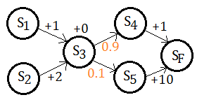 For $S_{F}$ is the state we end up in, this final state is set to $0$ in its value. As to other states, it’s the expected value of the reward plus the discounted value of the state we end up in.
$V(S)$=
➀$0$ for $S_{F}$.
➁$E\lbrack R_{i}+\gamma\cdot V(S’)\rbrack$, $S’$ is the state we arrive in.
The immediate reward associated are $+1$ with $S_{1}$, $+2$ with $S_{2}$, $0$ with $S_{3}$, $+1$ with $S_{4}$ and $+10$ with $S_{5}$. Let discounted factor $\gamma$=$1$, what is V($S_{3}$)?
[Answer]
We’d like to use the backup propagation to figure out the value function of these states:
➀V($S_{4}$)=$1$+$\gamma\cdot 1\cdot 0$=$1$
➁V($S_{5}$)=$10$+$\gamma\cdot 1\cdot 0$=$10$
➂V($S_{3}$)=$0$+$\gamma\cdot(0.9\cdot 1+0.1\cdot 10)$
=$1.9$, where $\gamma$=$1$
➃V($S_{1}$)=$1$+$\gamma\cdot 1\cdot 1.9$=$2.9$
➄V($S_{2}$)=$2$+$\gamma\cdot 1\cdot 1.9$=$3.9$
Estimate From Data In Example
[Question]
Given the same Markov chain with $\gamma$=$1$, this is the simulation before we know the whole image of the model.
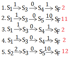
We'd like to estimate the value of $S_{1}$ after 3 and 4 episodes
, since nothing related to $S_{2}$, just ignore it.
[Hints]::by mjtsai1974
The red marked numbers are the value of $S_{1}$ in each episode. By using backup or expect discounted reward could we obtain the same value function of states, even for $\gamma$=$0.9$. Let me do the illustrtation of the 1st episode.
[1]by using backup:
➀$V(S_{4})$=$1+\gamma\cdot 1\cdot 0$
$V(S_{4})$=1 for $\gamma$=$1$ and $0.9$, where $\gamma\cdot 1$, this 1 is the probabilistic transition, since it's the only one path, the probability is $1$.
➁$V(S_{3})$=$0+\gamma\cdot V(S_{4})$
$V(S_{3})$=$1$ for $\gamma$=$1$ and $0.9$ for $\gamma$=$0.9$
➂$V(S_{1})$=$1+\gamma\cdot V(S_{3})$
$V(S_{1})$=$2$ for $\gamma$=$1$ and $1.81$ for $\gamma$=$0.9$
[2]by using expect discounted reward:
➀$V(S_{1})$ expression
=$1$+$\gamma\cdot 1\cdot(0+\gamma\cdot 1\cdot(1+\gamma\cdot 1\cdot 0))$
, where $V(S_{1})$=$2$ for $\gamma$=$1$ and $1.81$ for $\gamma$=$0.9$
[Answer]
The appropriate estimate for $V(S_{1})$ after 3 and 4 episodes would be $\frac {2+11+2}{3}$=$5$ and $\frac {2+11+2+2}{4}$=$4.25$ respectively.
To estimate from data is asking to do an expectation, it is just averaging things. We can incrementally compute an estimate for the value of a state, given the previous estimate.
But, it is a big jump for $V(S_{1})$ from $5$ to $4.25$, when it is estimated from eposide 3 to 4. With an inifinite amount of data in an already known Markov chain model, we should get $V(S_{1})$=$2.9$, which is the converged value, could be found in above section ReCap The Backup In Markov Chain.
Because, not enough data, just 3 episodes, an over-representation of the higher reward, that’s why we have higher skewed estimate of $5$ than $4.25$ in 4 episodes.
Computing Estimates Incrementally
[Question]
From prior example, we have the value of $S_{1}$=$5$, say $V_{3}(S_{1})$ after 3 episodes, then we ran an eposide, and the return of the episode, the total discounted reward of $S_{1}$ in this distinct 4-th sequence was $2$, say $R_{4}(S_{1})$.
Could we figure out what the new estimate of value of $S_{1}$, say $V_{4}(S_{1})$
, just from this information?
[Answer]
By weighting, $\frac {3\cdot 5 + 1\cdot 2}{4}$=$4.25$, we could get the same estimate identical to the way of expectation.
[The generalization]
Can we generalize it? Yes!
$V_{T}(S_{1})$
=$\frac {(T-1)\cdot V_{T-1}(S_{1})+1\cdot R_{T}(S_{1})}{T}$
=$\frac {(T-1)\cdot V_{T-1}(S_{1})}{T}$+$\frac {1\cdot R_{T}(S_{1})}{T}$
=$\frac {(T-1)\cdot V_{T-1}(S_{1})}{T}$+$\frac {V_{T-1}(S_{1})}{T}$+$\frac {1\cdot R_{T}(S_{1})}{T}$-$\frac {V_{T-1}(S_{1})}{T}$
=$V_{T-1}(S_{1})$+$\alpha_{T}\cdot (R_{T}(S_{1})-V_{T-1}(S_{1}))$
, where we have it that:
➀$\alpha_{T}$=$\frac {1}{T}$, the learning rate(parameter)
➁the temporal difference is the difference between the reward we get at this step and the estimate we had at th eprevious step.
➂$R_{T}(S_{1})-V_{T-1}(S_{1})$ is the error term. If the difference is zero, then no change; if the difference is (big) positive, then, it goes up; if the difference is big negative, then, it goes down.
As we get more and more eposides, this learning parameter $\alpha_{T}$ is getting small and small, and making smaller and smaller changes. It’s just like the update rule in perceptrons learning and neural network learning.
The Property Of Learning Rate
By given $V_{T}(S)$=$V_{T-1}(S)$+$\alpha_{T}\cdot(R_{T}(S)-V_{T-1}(S))$, then, $\lim_{T\rightarrow\infty}V_{T}(S)$=$V(S)$, with below 2 properties guarantee the convergence:
➀$\sum_{T=0}^{\infty}\alpha_{T}\rightarrow\infty$
➁$\sum_{T=0}^{\infty}(\alpha_{T})^{2}<\infty$
proof::mjtsai1974
I’d like to prove the learning rate property by using geometric series convergence/divergence by Gilbert Strange in Calculus.
➀begin from $T$=$0$, initially $V_{0}(S)$=$C$, some constant, might be zero. And $V_{T}(S)$=$V_{T-1}(S)$=$V_{0}(S)$ at this moment.
➁suppose the equality holds, then expand from $T+1$:
$V_{T+1}(S)$
=$V_{T}(S)$+$\alpha_{T}\cdot(R_{T+1}(S)-V_{T}(S))$
=$V_{T}(S)$+$\alpha_{T}\cdot(R_{T+1}(S)-(V_{T-1}(S)$+$\alpha_{T}\cdot(R_{T}(S)-V_{T-1}(S))))$
=$V_{T}(S)$+$\alpha_{T}\cdot(R_{T+1}(S)-(V_{T-1}(S)$+$\alpha_{T}\cdot(R_{T}(S)-(V_{T-2}(S)$+$\alpha_{T}\cdot(R_{T-1}(S)-V_{T-2}(S))))))$
➂the expand could be continued, but we stop over here for our proof…
=$V_{T}(S)$+$\alpha_{T}\cdot(R_{T+1}(S)-V_{T-1}(S))$
$\;\;$+$\alpha_{T}^{2}\cdot(R_{T}(S)-V_{T-2}(S))$
$\;\;$+$\alpha_{T}^{3}\cdot(R_{T-1}(S)-V_{T-2}(S))$
➃to make it perfect, expand the term $V_{T-2}(S)$, we can get it down the way to $T=0$:
=$V_{T}(S)$+$\alpha_{T}\cdot(R_{T+1}(S)-V_{T-1}(S))$
$\;\;$+$\alpha_{T}^{2}\cdot(R_{T}(S)-V_{T-2}(S))$
$\;\;$+$\alpha_{T}^{3}\cdot(R_{T-1}(S)-V_{T-3}(S))$
$\;\;$+$\alpha_{T}^{4}\cdot(R_{T-2}(S)-V_{T-4}(S))$
$\;\;$+$\alpha_{T}^{5}\cdot(R_{T-3}(S)-V_{T-5}(S))$+…
➄we take $E_{1}$=$R_{T+1}(S)-V_{T-1}(S)$
$\;\;\;\;E_{2}$=$R_{T}(S)-V_{T-2}(S)$
$\;\;\;\;E_{3}$=$R_{T-1}(S)-V_{T-3}(S)$
…
, where each $E_{i}$ is a constant, assume they are rather stable, non-variant, then we take these error terms as $E$.
➅then, the whole terms after the first + operator could be expressed as:
$\alpha_{T}\cdot E$+$\alpha_{T}^{2}\cdot E$+$\alpha_{T}^{3}\cdot E$+$\alpha_{T}^{4}\cdot E$+…
=$(\alpha_{T}+\alpha_{T}^{2}+\alpha_{T}^{3}+\alpha_{T}^{4}+…)\cdot E$
=$(\lim_{k\rightarrow\infty}\sum_{i=1}^{k}\alpha_{T}^{i})\cdot E$, then,
$\lim_{k\rightarrow\infty}\sum_{i=1}^{k}\alpha_{T}^{i}$=$\frac {\alpha_{T}}{1-\alpha_{T}}$, for $\left|\alpha_{T}\right|$<$1$, and it holds to have these 2 properties, it is the convergent series, you can see in my prior post Series Convergence.
The $TD(\lambda)$ Algorithm
[The rule]
Eposide $T$:
$\;\;$For all $S$, $e(S)$=$0$ at start of eposide, $V_{T}(S)$=$V_{T-1}(S)$
$\;\;$After $S_{t-1}\xrightarrow{r_{t}}S_{t}$:(from step $t-1$ to $t$ with reward $r_{t}$)
$\;\;\;e(S_{t-1})$=$e(S_{t-1})$+$1$:
$\;\;\;\;$Update eligibility of $S_{t-1}$ after arriving to $S_{t}$
$\;\;$For all $S$,
$\;\;V_{T}(S)$=$V_{T-1}(S)$+$\alpha_{T}\cdot(r_{t}+\gamma\cdot V_{T-1}(S_{t})-V_{T-1}(S_{t-1}))$
$\;\;\;e(S_{t-1})$=$\lambda\cdot\gamma\cdot e(S_{t-1})$:
$\;\;\;\;$before transite from $S_{t-1}$ to $S_{t}$ in next iteration
[Notes]
Where the $T$ stands for the specific eposide, $t$ is the index for state transition, and $e(S_{t})$ is for the eligibility.
$TD(1)$ Algorithm: $\lambda$=$1$
This is by taking $\lambda$=$1$ in $TD(\lambda)$ algorithm.
[The rule]
Eposide $T$:
$\;\;$For all $S$, $e(S)$=$0$ at start of eposide, $V_{T}(S)$=$V_{T-1}(S)$
$\;\;$After $S_{t-1}\xrightarrow{r_{t}}S_{t}$:(from step $t-1$ to $t$ with reward $r_{t}$)
$\;\;\;e(S_{t-1})$=$e(S_{t-1})$+$1$:
$\;\;\;\;$Update eligibility of $S_{t-1}$ after arriving to $S_{t}$
$\;\;$For all $S$,
$\;\;V_{T}(S)$=$V_{T-1}(S)$+$\alpha_{T}\cdot(r_{t}+\gamma\cdot V_{T-1}(S_{t})-V_{T-1}(S_{t-1}))$…[A]
$\;\;\;e(S_{t-1})$=$\gamma\cdot e(S_{t-1})$:
$\;\;\;\;$before transite from $S_{t-1}$ to $S_{t}$ in next iteration
[Notes]
➀the 2nd part of [A] is sum of the reward plus the the discounted value of the state we just arrived, minus the state value we just left; where these state values are all evaluated in last iteration. It could just be the temporal difference.
➁we are going to apply the temporal difference onto all states, proportional to the eligibility of each distinct state, and the learning rate would be specified for we don’t want it to move too much.
➂after the state has been iterated, decay or decrease its eligibility with $\lambda\cdot\gamma$, in their given value, in $TD(1)$, $\lambda$=$1$.
➃and we are backing up to next state.
[Caution]
➀all the $S$ are all being done in similar approach.
➁the value at state $S$(the $S$ in (A)) is going to be updated on this quantity, $r_{t}+\gamma\cdot V_{T-1}(S_{t})-V_{T-1}(S_{t-1})$, which is the same for everybody, doesn't depend on which $S$ we are updating, and $e(S)$ is specific to the state $S$ we are evaluating(looking at).
Example: $TD(1)$ Illustration
[1]
Keeping track of changes ultimately
Let’s walk through the pseudo code in this given example, just to see how value update works.
 ➀we are starting off at the beginning of an eposide. Now, the eligibility for all states are all zero.
➁we’d like to keep track of changes ultimately, it’s all going to get added to whatever the previous value.
➂the 1st transition is from $S_{1}$ to $S_{2}$ with reward $r_{1}$, and sets the eligibility $e(S_{1})$ to 1 for $S_{1}$.
➃we’d like to loop through all the states, all of them, and apply the same little update to all of the states.
[2]
The expression of the update
The update has the form:
➀whatever the current learning rate is, times the reward which we just experienced, say $r_{1}$, plus the discount factor gamma $\gamma$ times the previous value of the state we newly arrived, minus the the previous value of the state we just left.
➁$\alpha_{T}\cdot(r_{t}+\gamma\cdot V_{T-1}(S_{t})-V_{T-1}(S_{t-1}))$, it is going to get added to all states, such quantity is proportional to the eligibility of that state.
[3]
The update from $S_{1}$ to $S_{2}$
After transiting from $S_{1}$ to $S_{2}$, at this moment, the eligibility of $S_{2}$ and $S_{3}$ are $0$, we are only making updating with respect to $S_{1}$.
 ➀$\triangle V_{T}(S_{1})$=$\alpha\cdot(r_{1}+\gamma\cdot V_{T-1}(S_{2})-V_{T-1}(S_{1}))$, where $\alpha_{T}$=$\alpha$ wichi is a constant all the way.
➁$\triangle V_{T}(S_{2})$=$0$
➂$\triangle V_{T}(S_{3})$=$0$
Before next step from $S_{2}$ to $S_{3}$, be sure to decay current evaluated state $S_{1}$'s eligibility by $\gamma$.
 This is the eligibility after $S_{1}$ to $S_{2}$.
[4]
The update from $S_{2}$ to $S_{3}$
We take next step from $S_{2}$ to $S_{3}$ with reward $r_{2}$. It bumps $S_{2}$'s eligibility from $0$ to $1$.
 Current eligibility at this moment are $\gamma$,$1$,$0$ for $S_{1}$,$S_{2}$,$S_{3}$. The update term $\alpha\cdot(r_{2}+\gamma\cdot V_{T-1}(S_{3})-V_{T-1}(S_{2}))$, is independent of which state we are actually changing, we are going to apply it with respect to each state's($S_{1}$,$S_{2}$) eligibility, proportionally.
➀$\triangle V_{T}(S_{1})$
=$\alpha\cdot(r_{1}+\gamma\cdot V_{T-1}(S_{2})-V_{T-1}(S_{1}))$
$\;\;+\gamma\cdot\alpha\cdot(r_{2}+\gamma\cdot V_{T-1}(S_{3})-V_{T-1}(S_{2}))$
=$\alpha\cdot(r_{1}+\gamma\cdot r_{2}+\gamma^{2}\cdot V_{T-1}(S_{3})-V_{T-1}(S_{1}))$
➁$\triangle V_{T}(S_{2})$=$\alpha\cdot(r_{2}+\gamma\cdot V_{T-1}(S_{3})-V_{T-1}(S_{2}))$
➂$\triangle V_{T}(S_{3})$=$0$
Before next step from $S_{3}$ to $S_{F}$, be sure to decay current already evaluated states $S_{1}$ and $S_{2}$'s eligibility by $\gamma$.
 This is the eligibility after $S_{2}$ to $S_{3}$.
[5]
The update from $S_{3}$ to $S_{F}$
Finally, we take next step from $S_{3}$ to $S_{F}$ with reward $r_{3}$. It bumps $S_{3}$'s eligibility from $0$ to $1$. Current eligibility at this moment are $\gamma^{2}$,$\gamma$,$1$ for $S_{1}$,$S_{2}$,$S_{3}$.
 The update term $\alpha\cdot(r_{3}+\gamma\cdot V_{T-1}(S_{F})-V_{T-1}(S_{3}))$, is independent of which state we are actually changing, we are going to apply it with respect to each state's($S_{1}$,$S_{2}$,$S_{3}$) eligibility, proportionally.
➀$\triangle V_{T}(S_{1})$
=$\alpha\cdot(r_{1}+\gamma\cdot V_{T-1}(S_{2})-V_{T-1}(S_{1}))$
$\;\;+\gamma\cdot\alpha\cdot(r_{2}+\gamma\cdot V_{T-1}(S_{3})-V_{T-1}(S_{2}))$
$\;\;+\gamma^{2}\cdot\alpha\cdot(r_{3}+\gamma\cdot V_{T-1}(S_{F})-V_{T-1}(S_{3}))$
=$\alpha\cdot(r_{1}+\gamma\cdot r_{2}+\gamma^{2}\cdot r_{3}+\gamma^{3}\cdot V_{T-1}(S_{F})-V_{T-1}(S_{1}))$
➁$\triangle V_{T}(S_{2})$
=$\alpha\cdot(r_{2}+\gamma\cdot V_{T-1}(S_{3})-V_{T-1}(S_{2}))$
$\;\;+\gamma\cdot\alpha\cdot(r_{3}+\gamma\cdot V_{T-1}(S_{F})-V_{T-1}(S_{3}))$
=$\alpha\cdot(r_{2}+\gamma\cdot r_{3}+\gamma^{2}\cdot V_{T-1}(S_{F})-V_{T-1}(S_{2}))$
➂$\triangle V_{T}(S_{3})$=$\alpha\cdot(r_{3}+\gamma\cdot V_{T-1}(S_{F})-V_{T-1}(S_{3}))$
Where we have the value of the state $S_{F}$ as $0$, at this ending, even no next state to jump to, we should also decrease each state's eligibility by $\gamma$.

[Notes]
➀$TD(1)$ is the same as the outcome-base update, that is to say we want to see all the discounted rewards on the entire trajectory, and we just update our prediction of the state that they started from with those rewards.
➁in this article, we are talking about the discounted sum of rewards minus the old prediction(evaluated in the last episode $T-1$).
Example: $TD(1)$ Illustration In Repeated States
[The case of repeated states]
 If we follow up $TD(1)$ rule, you might get:
$\triangle V_{T}(S_{F})$=$\alpha\cdot(r_{1}’$+$\gamma\cdot V_{T-1}(S_{F})-V_{T-1}(S_{1}))$
➀the online course said that it a mistake, for you go to $S_{1}$, you saw $S_{1}$ transite to $S_{2}$ with $r_{1}$, therefore you just ignore anything you learned along the way.
➁the $TD(1)$ rule lets you do is, when you see $S_{1}$ again, and sort of backup its value, you’re actually capturing the fact the last time you were in $S_{1}$, you actually went to $S_{2}$ and saw $r_{1}$.
➂it’s just like outcome-base on updates, now with extra learning or inside the eposide learning from head of the trajectory.
[But, mjtsai's viewpoint]
Suppose you have just completed the 1st run and reach $S_{F}$, now you are transiting to $S_{1}$ again, the eligibility of all states and state transition diagram are given in below:
 Such eligibility is not yet in the ending of this transition, it is in the beginning. If you complete the transition and would like to start to transit from $S_{1}$ to $S_{2}$, be sure to remember to decay all the eligibility by $\gamma$, guess what, it should be $\gamma^{4}$,$\gamma^{3}$,$\gamma^{2}$,$\gamma$ for $S_{1}$,$S_{2}$,$S_{3}$,$S_{F}$.
➀the update term of $S_{F}$ in eposide $T$:
$\triangle V_{T}(S_{F})$=$\alpha\cdot(r_{1}’$+$\gamma\cdot V_{T-1}(S_{1})-V_{T-1}(S_{F}))$
➁the update term of $S_{1}$ when transiting from $S_{F}$ to $S_{1}$:
$\triangle V_{T+1}(S_{1})$
=$\triangle V_{T}(S_{1})$+$laerning\;rate\cdot e(S_{1})\cdot\triangle V_{T}(S_{F})$
=$\alpha\cdot(r_{1}+\gamma\cdot r_{2}+\gamma^{2}\cdot r_{3}+\gamma^{3}\cdot V_{T-1}(S_{F})-V_{T-1}(S_{1}))$
$\;\;+\alpha\cdot\gamma^{3}\cdot(r_{1}’$+$\gamma\cdot V_{T-1}(S_{1})-V_{T-1}(S_{F}))$
; where the $\triangle V_{T+1}(S_{1})$ term is the initial temporal difference of $S_{1}$ in the beginning of eposide $T+1$, while $\triangle V_{T}(S_{1})$=$0$ is the initial update term in the beginning of eposide $T$, if we treat eposide $T$ the very first eposide in this case of repeated states.
➂the update term of $S_{1}$ when transiting from $S_{F}$ to $S_{1}$, in the eposide $T$ to $T+1$(the very 1st repeat) could be:
$\alpha\cdot(r_{1}+\gamma\cdot r_{2}+\gamma^{2}\cdot r_{3}+\gamma^{3}\cdot r_{1}’-V_{T-1}(S_{1})\cdot(1-\gamma^{4}))\cdot\gamma^{0}$
, then in the eposide $T+n-1$ to $T+n$(the n-th repeat) could becomes:
$\alpha\cdot(r_{1}+\gamma\cdot r_{2}+\gamma^{2}\cdot r_{3}+\gamma^{3}\cdot r_{1}’-V_{T+n-2}(S_{1})\cdot(1-\gamma^{4}))\cdot\gamma^{n-1}$
, this says in the n-th repeat, the update term of $S_{1}$ in this example should be:
$\alpha\cdot(r_{1}+\gamma\cdot r_{2}+\gamma^{2}\cdot r_{3}+\gamma^{3}\cdot r_{1}’-V_{T+n-2}(S_{1})\cdot(1-\gamma^{4}))\cdot\gamma^{n-1}$
From above deduction, we can say that the repeated state influence on temporal difference depends on how far it is to be repeated, that is how many state changes in between the repeated state, the longer the smaller the impact it is!!
Also, the number of times the trajectory has been repeated is a factor expressed in term of $\gamma$ with the exponent of this number minus 1.
[The repeated update term of $S_{2}$::mjtsai1974]
I’d like to generalize the expression of update term of $S_{2}$ in the repeated case. Below exhibits the eligibility upgrade in the 1st repeation of $S_{2}$.
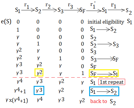 Next to investigate the update term of $S_{2}$, the initial temporal difference of $S_{2}$ in eposide $T+1$ consists of below 3 parts:
➀$\alpha\cdot(r_{2}$+$\gamma\cdot r_{3}$+$\gamma^{2}\cdot V_{T-1}(S_{F})-V_{T-1}(S_2))$
This is the part of update term of $S_{2}$ after transiting to $S_{F}$, in eposide $T$.
➁$\alpha\cdot\gamma^{2}\cdot(r_{1}’+\gamma\cdot V_{T-1}(S_{1})-V_{T-1}(S_{F}))$
This is the part of update term of $S_{2}$ contributed from $S_{F}$ to $S_{1}$, be noted that the eligibility of $S_{2}$ is $\gamma^{2}$ at this moment in eposide $T$.
➂$\alpha\cdot\gamma^{3}\cdot(r_{1}+\gamma\cdot V_{T}(S_{2})-V_{T}(S_{1}))$
This is the part of update term of $S_{2}$ contributed when transiting from $S_{1}$ to $S_{2}$ in eposide, watch out, it’s $T+1$ now, thus, we use $V_{T}(S_{1})$, $V_{T}(S_{2})$. The eligibility of $S_{2}$ at this moment is $\gamma^{3}$.
Next to add up ➀,➁,➂, we get this expression:
$\triangle V_{T+1}(S_{2})$
=$\alpha\cdot(r_{2}+\gamma\cdot r_{3}+\gamma^{2}\cdot r_{1}’+\gamma^{3}\cdot r_{1}$
$\;\;$+$\gamma^{4}\cdot V_{T}(S_{2})-V_{T-1}(S_{2})$
$\;\;$+$\gamma^{3}\cdot V_{T-1}(S_{1})-\gamma^{3}\cdot V_{T}(S_{1}))$…[A]
Can we treat $\gamma\cdot V_{T}(S_{2})\approx V_{T-1}(S_{2})$? Suppose we'd like to decay in a linear, gentle fashion, and $\gamma\rightarrow 1$, after a period of some horizon, the value of a state would just converge, therefore, above expression becomes:
$\alpha\cdot(r_{2}+\gamma\cdot r_{3}+\gamma^{2}\cdot r_{1}’+\gamma^{3}\cdot r_{1}$
$\;\;$-$V_{T-1}(S_{2})(1-\gamma^{3})$
$\;\;$+$\gamma^{3}\cdot (V_{T-1}(S_{1})-V_{T}(S_{1})))$
, where $V_{T-1}(S_{1})\rightarrow V_{T}(S_{1})$ after some period of time, $V_{T-1}(S_{1})-V_{T}(S_{1})\approx 0$ is reasonable, this term could be safely tossed out.
However, we are talking about the initial temporal difference of $S_2$ in eposide $T+1$, we should evaluate on the value of $S_{2}$ in eposide $T$. Therefore, back to [A], this time, we choose $V_{T}(S_{2})\approx V_{T-1}(S_{2})$, this holds for convergence. The whole equation becomes:
$\alpha\cdot(r_{2}+\gamma\cdot r_{3}+\gamma^{2}\cdot r_{1}’+\gamma^{3}\cdot r_{1}$
$\;\;$-$V_{T}(S_{2})(1-\gamma^{4}))$
It is just the update term of $S_{2}$, $\triangle V_{T+1}(S_{2})$ after its 1st repeat, the same manner as it is in $S_{1}$!!
This says in the n-th repeat, the update term of $S_{2}$ in this example should be:
$\alpha\cdot(r_{2}+\gamma\cdot r_{3}+\gamma^{2}\cdot r_{1}’+\gamma^{3}\cdot r_{1}$
$\;\;$-$V_{T+n-1}(S_{2})(1-\gamma^{4}))\cdot\gamma^{n-1}$
[The formal expression of the update term in repeated case::mjtsai1974]
Here, I’d like to make this claim, for the trajectory containing states $\{S_{1}$,$S_{2}$,…,$S_{k}\}$ with the repeated path from $S_{k}$ to $S_{1}$, the update term of $S_{i1}$ in the n-th repeat could be generalized in below expression:
$\alpha\cdot(r_{i1}+\gamma\cdot r_{i2}+\gamma^{2}\cdot r_{i3}$
+$…+\gamma^{k-1}\cdot r_{ik}-V_{T+n-1}(S_{i1}))\cdot \gamma^{n-1}$, where
$(i1,i2,…,ik)$
=$\{(1,2,3,…,k),$
$\;(2,3,…,k-1,k,1),$
$\;(3,4,…,k,1,2),$
…
$(k,1,2,…,k-2,k-1)\}$
[Cautions]
Cautions must be made that there exists some other alternative for the deduction of update term expression in repeated case, to be conti in the incoming future.
Addendum
➀Temporal Difference Learning, Charles IsBell, Michael Littman, Reinforcement Learning By Georgia Tech(CS8803)
12 Nov 2018
Prologue To The Calibrated Clique Tree
The quantitative evaluation of messages from one clique to its adjacent clique and from this adjacent clique to itself would be a equilibrium in a calibrated clique tree.
Before We Go Any Farther
[1]
Recap: variable-elimination constructed clique tree
Remember that my prior post The Clique Tree Construction has proved that slight different and very different elimination order constructed clique tree makes the same propagation.
[2]
Recap: message passing in the clique tree
Still in another prior post of mine, The Bayesian Network Propagation And Clique Tree:
➀the message propagation in the clique tree is proceeded in two stage operations with the former the collection(from leaf nodes to the pivot node) and the next is the distribution(from pivot node to the leaf nodes).
➁computation sharing in all queries that the function of the message from the pivot to the leafs are all expressed in terms of the variables the same as it is in the clique from which passes message to the pivot.
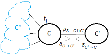
➂given clique $C$ and $C’$ in adjacent, there exists $C_{i}$ for $i$=$1$ to $k$ to be $C$’s neighbors, $g_{i}$ is the message from $C_{i}$ to $C$, and $f_{j}$ is the $j$-th function attached to clique $C$, the message from $C$ to $C’$ is denoted as $H$, expressed as:
$H((C\cap C’)-E)$=$\sum_{C\backslash C’\cup E}\prod_{i}g_{i}\prod_{j}f_{j}$, with $E$ to be the evidence.
The summation over elements purely from $C$
, not belonging to $C’$ and $E$(evidence), then:
$H((C\cap C’)-E)$=$\sum_{C\backslash C\cap C’}\prod_{i}g_{i}\prod_{j}f_{j}$ also holds for it sums out the variables only in $C$!!
The term $(C\cap C’)-E$ illustrates that the message purely propagates from $C$ to $C’$, exclusive of the intermediate noise.
[3]
Notes
The clique tree is also called a junction tree or a join tree.
What Is The Calibrated Clique Tree?
[1]
Run message passing with each clique in the tree as the pivot(root)
Suppose you have a well constructed clique tree:
➀take one clique that neither has been used as a pivot nor all its containing variables has been belief updated.
➁run message passing from leave nodes to this pivot node with one variable chosen for belief update(such variable must not have been propagated with message in this clique).
➂in the message passing from one clique to another, marginalizes over variables other than ➁ chosen variable, thus to have the final factor containing only this variable in it.
➃repeat ➀ until each clique and all variables in it has been belief updated.
[2]
The calibrated clique tree
After each clique with all its variables has been belief updated, we will have a calibrated clique tree if below condition is satisfied:
$\;\;\sum_{C_{i}\backslash S_{i,j}}Bel_{i}$=$\sum_{C_{j}\backslash S_{i,j}}Bel_{j}$
where,
➀we denote $Bel_{i}$ for the belief update on clique $i$.
➁we take $S_{i,j}$=$C_{i}\cap C_{j}$ as the edge in between $C_{i}$ and $C_{j}$.
➂$C_{i}$ and $C_{j}$ are any two adjacent cliques in the tree.
➃we say that $C_{i}$ and $C_{j}$ are calibrated.
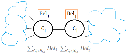 We can also use $Bel_{i}(X)$ to be the posterior belief update of variable $X$ in clique $i$; for the simplicity, the belief update would be proceeded in the unit of each distinct clique in this article.
Illustrtation Of The Calibrated Clique Tree::by mjtsai1974
[1]
From BN to MN
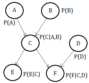 Suppose we are given this BN, with probability distributed over each variable:
➀the total joint probability would be
$P(A,B,C,D,E,F)$
=$P(F\vert C,D)\cdot P(E\vert C)\cdot P(D)$
$\;\;P(C\vert A,B)\cdot P(B)\cdot P(A)$
➁we’d like to query for $P(A,B,C\vert d,e,f)$=$\frac {P(A,B,C,d,e,f)}{\sum_{A,B,C}P(A,B,C,d,e,f)}$, under the observation(evidence) that $D$=$d$,$E$=$e$,$F$=$f$.
➂moralize it, we get below MN.
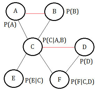
[2]
Construct the clique tree
By using the variable elimination order $A,B,E,F,D,C$, we construct this clique tree:
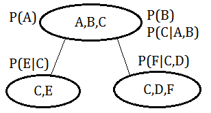 ➀we choose the clique $(A,B,C)$ as the pivot, for the 1st phase of collection:
$f_{2}(C)$=$\sum_{E}P(E\vert C)$
$f_{3}(C)$=$\sum_{D,F}P(D)\cdot P(F\vert C,D)$
$f_{1}(A,B,C)$=$P(A)\cdot P(B)\cdot P(C\vert A,B)$
$f_{0}(A,B,C)$=$f_{3}(C)\cdot f_{2}(C)\cdot f_{1}(A,B,C)$
, where $f_{0}(A,B,C)$ is the final collected messages in the clique $(A,B,C)$.
➁in the 2nd phase of distribution, from the pivot to the leafs:
$f_{4}(C,E)$=$f_{3}(C)\cdot(\sum_{A,B}f_{1}(A,B,C)\cdot P(E\vert C))$
$f_{5}(C,D,F)$=$P(D)\cdot P(F\vert C,D)$
$\;\;\cdot(\sum_{A,B}f_{1}(A,B,C)\cdot f_{2}(C))$
, where $f_{4}(C,E)$ is the message from pivot to $(C,E)$, and $f_{5}(C,D,F)$ is the message from pivot to $(C,D,F)$.
$f_{0}(A,B,C)$ in the collection phase, $f_{4}(C,E)$ and $f_{5}(C,D,F)$ in the distribution phase are all operating over the same factors.
Although the computation of $f_{0}(A,B,C)$, $f_{4}(C,E)$ and $f_{5}(C,D,F)$ are using the same factors, the marginalizations in these 2 phase are proceeded over different variables, which doesn't guarantee to have the equivalent posterior belief
.
[3]
The proof of the calibrated clique tree
When $C_{i}$ and $C_{j}$ are calibrated, $\sum_{C_{i}\backslash S_{i,j}}Bel_{i}$=$\sum_{C_{j}\backslash S_{i,j}}Bel_{j}$.
proof::mjtsai1974
Succeesding to above:
➀take $Bel_{1}$=$f_{0}(A,B,C)$ for the belief updated in clique $C_{1}$.
➁take $Bel_{2}$=$f_{4}(C,E)$ for the belief updated in clique $C_{2}$.
➂take $Bel_{3}$=$f_{5}(C,D,F)$ for the belief updated in clique $C_{3}$.
➃then we have below equilibrium holds:
$\sum_{A,B}Bel_{1}$=$\sum_{E}Bel_{2}$
$\sum_{A,B}Bel_{1}$=$\sum_{D,F}Bel_{3}$
[4]
The expression of the calibrated message
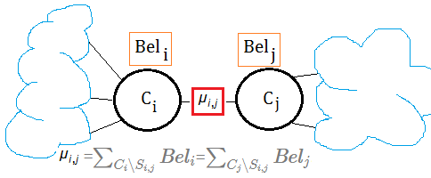 ➀take $\mu_{i,j}$ to be the calibrated message from clique $i$ to clique $j$.
➁still using the same example, $\mu_{1,2}$ is the calibrated message from clique $1$ to clique $2$, then
$\mu_{1,2}$
=$\sum_{A,B}Bel_{1}$
=$\sum_{A,B}f_{3}(C)\cdot f_{2}(C)\cdot f_{1}(A,B,C)$
=$\sum_{A,B}f_{3}(C)\cdot f_{1}(A,B,C)\cdot f_{2}(C)$
=$(\sum_{A,B}f_{3}(C)\cdot f_{1}(A,B,C))\cdot (\sum_{E}P(E\vert C))$
=$\delta_{1,2}\cdot\delta_{2,1}$
, where $delta_{i,j}$ is the before-calibrated message propagated from clique $i$ to clique $j$.
➂$\mu_{1,3}$=$\delta_{1,3}\cdot\delta_{3,1}$ could also be proved, by mathematics induction, we can claim that $\mu_{i,j}$=$\delta_{i,j}\cdot\delta_{j,i}$.
The calibrated message from clique $i$ to clique $j$ is the joint probability function of the before-calibrated message from clique $i$ to clique $j$ and the before-calibrated message from clique $j$ to clique $i$
.
[5]
The generalization of the calibrated message

proof::mjtsai1974
➀take $neighbor(C)$=${C”}\cup{C’}$
➁take $\mu_{S=C\cap C’}$ te be the calibrated message from clique $C$ to $C’$(or $C’$ to $C$), then
$\mu_{S=C\cap C’}$
=$\sum_{C\backslash S}\prod f_{j}\prod_{C”\in neighbor(C)}\delta_{C”\rightarrow C}$
=$\sum_{C\backslash S}\prod f_{j}\prod_{C”\in neighbor(C)\backslash C’}\delta_{C”\rightarrow C}$
$\;\;\cdot \delta_{C’\rightarrow C}$
=$\delta_{C\rightarrow C’}\cdot \delta_{C’\rightarrow C}$
, where $f_{j}$ is the function attached to clique $C$.
➂if we choose the calibrated message from clique $C$ to $C’$, then we have
$\mu_{C,C’}$
=$\delta_{C\rightarrow C’}\cdot \delta_{C’\rightarrow C}$
and, it also hods for below
$\mu_{C’,C}$
=$\delta_{C’\rightarrow C}\cdot \delta_{C\rightarrow C’}$
Before The End Of Bayesian Network Begin@20181201
[1]
Brief summary
Using Bayesian network to compute probability of the query in the form of $P(X\vert E)$ is called inference, where $E$ is the observed evidence variable(s), $X$ is the query variable(s) in the network.
The Bayesian networks are useful for these tasks:
➀diagnosis of the form $P(causes\vert symptom)$, the quantitative thinking.
➁predict of the form $P(symptom\vert causes)$, the qualitative thinking.
➂classification of the form $\underset{class}{max}P(class\vert data)$.
➃decision making by given/develop certain kind of cost function in a subsystem.
I have ➀ and ➁ involved in a lot of my previous posts, in the incoming future, I expect myself to investigate ➂ and ➃, you can find some future direction in p.11~43 of A Tutorial on Inference and Learning in Bayesian Networks, Irina Rish, IBM T.J.Watson Research Center.
[2]
Time to back to Reinforcement Learning
In the early May of 2018, I was struggling over reinforcement learning in exploitation versus exploration, for some terminology, prior or posterior alike, I explore to the Bayesian network, after months of exploitation, I should resume my reinforcement learning and explore to next station of unknow, maybe sooner or later involved in the Bayesian network due to this deep exploitation in these days.
Finally, the Bayesian network network is a network of multiple variables, while reinforcement learning is a network of only one variable iterating over multiple states.
Addendum
➀Graphical Models - Lecture 11: Clique Trees, Andrew McCallum, mccallum@cs.umass.edu
➁A Tutorial on Inference and Learning in Bayesian Networks, Irina Rish, IBM T.J.Watson Research Center


 For $S_{F}$ is the state we end up in, this final state is set to $0$ in its value. As to other states, it’s the expected value of the reward plus the discounted value of the state we end up in.
 ➀we are starting off at the beginning of an eposide. Now, the eligibility for all states are all zero.
 ➀$\triangle V_{T}(S_{1})$=$\alpha\cdot(r_{1}+\gamma\cdot V_{T-1}(S_{2})-V_{T-1}(S_{1}))$, where $\alpha_{T}$=$\alpha$ wichi is a constant all the way.
  This is the eligibility after $S_{1}$ to $S_{2}$.
 Current eligibility at this moment are $\gamma$,$1$,$0$ for $S_{1}$,$S_{2}$,$S_{3}$. The update term $\alpha\cdot(r_{2}+\gamma\cdot V_{T-1}(S_{3})-V_{T-1}(S_{2}))$, is independent of which state we are actually changing, we are going to apply it with respect to each state's($S_{1}$,$S_{2}$) eligibility, proportionally.
 This is the eligibility after $S_{2}$ to $S_{3}$.
 The update term $\alpha\cdot(r_{3}+\gamma\cdot V_{T-1}(S_{F})-V_{T-1}(S_{3}))$, is independent of which state we are actually changing, we are going to apply it with respect to each state's($S_{1}$,$S_{2}$,$S_{3}$) eligibility, proportionally.
 If we follow up $TD(1)$ rule, you might get:
 Such eligibility is not yet in the ending of this transition, it is in the beginning. If you complete the transition and would like to start to transit from $S_{1}$ to $S_{2}$, be sure to remember to decay all the eligibility by $\gamma$, guess what, it should be $\gamma^{4}$,$\gamma^{3}$,$\gamma^{2}$,$\gamma$ for $S_{1}$,$S_{2}$,$S_{3}$,$S_{F}$.
 Next to investigate the update term of $S_{2}$, the initial temporal difference of $S_{2}$ in eposide $T+1$ consists of below 3 parts:
 We can also use $Bel_{i}(X)$ to be the posterior belief update of variable $X$ in clique $i$; for the simplicity, the belief update would be proceeded in the unit of each distinct clique in this article.
 Suppose we are given this BN, with probability distributed over each variable:
 ➀we choose the clique $(A,B,C)$ as the pivot, for the 1st phase of collection:
 ➀take $\mu_{i,j}$ to be the calibrated message from clique $i$ to clique $j$.