14 Oct 2018
Prologue To The Clique Tree Construction
The construction of clique tree aims at minimal cliques with none of them being the subsets of their neighbors, by using VE(variable elimination) in moral graph.
VE Versus Clique Tree Propagation
In my early post Variable Elimination Order And Moral Graph, we have explored how to query non-directly connected variables in the BN by means of VE and have a clear mapping in the MN. In advance to construct the clique tree, recap the VE and make comparison with clique tree propagation.
[1]
Variable elimination
➀answers one query at a time, for query of other variables, the whole VE must be proceeded.
➁delete non-queried variables during VE process.
➂no computation sharing among different queries.
[2]
Clique tree propagation
➀make posterior belief update for all variables, inclusive of these un-observed variables.
➁delete no any variable in the propagation of message passing.
➂allows computation sharing among different queries.
Since clique tree propagation could be distributed on un-observed variables, empirical results suggest to use it when we’d like to make posteriro belief update on un-observed variables.
Clique Tree Construction Algorithm
[1]
Target
Given a BN, the target would be:
➀construct a clique tree that covers the BN, with its clique be the smallest.
➁by using VE in the moral graph as the solution.
[2]
Algorithm
There exists over a dozen of clique tree construction algorithm, I list one workable and rather simple workflow, from Introduction to Bayesian Networks, Lecture 5: Inference as Message Propagation, Nevin L. Zhang, lzhang@cse.ust.hk, Department of Computer Science and Engineering, Hong Kong University of Science and Technology, Fall 2008, all related illustration in this article are under progress of this algorithm.
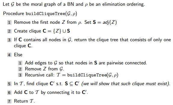 In the incoming future, I might have my own version of algorithm.
[3]
Illustration by example
Given the same BN, suppose the elimination order is $X,A,S,D,B,L,T,R$, proceed with the following steps:
➀moralize the BN to get the MN.
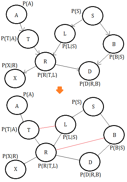 ➁eliminate variable $X$, we get the clique $(X,R)$:
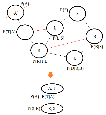
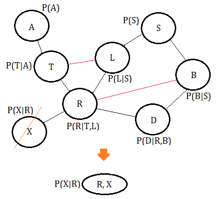 ➂eliminate variable $A$, we get the clique $(A,T)$:
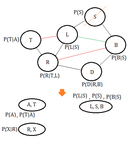
 ➃eliminate variable $S$, we get the clique $(L,S,B)$, where the green line is the new pairwise connection after $S$ has been removed:
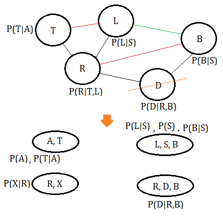
 ➄eliminate variable $D$, we get the clique $(R,D,B)$:
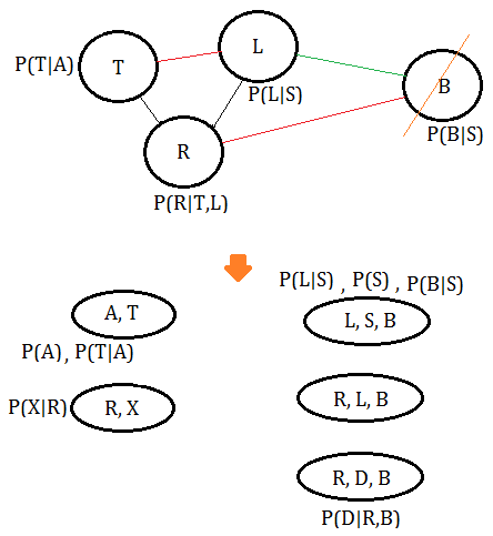
 ➅eliminate variable $B$, we get the clique $(L,R,B)$:
 ➆eliminate variable $L$, we get the final clique $(T,L,R)$:
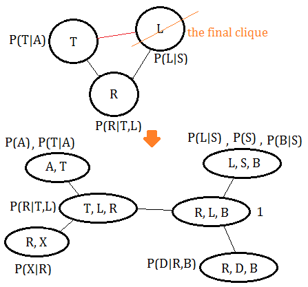 Finally, connect the cliques thus obtained in accordance to the moralized MN.
[4]
The clique tree is not unique
➀will the different elimination order construct clique tree identical to the moralized MN, or the original BN?
➁the clique tree is not unique, if we are using different elimination orders.
Due to above concern, will the posterior belief update all the same in the clique tree thus constructed, versus VE? I will prove my answer in the following sections.
Slight Different Elimination Order Constructed Clique Tree Makes The Same Propagation::by mjtsai1974
In this section, I’d like to prove that constructing clique tree by using slight different elimination order would just make the same propagation.
[Question]
Suppose we are give the same above BN, this time, the elimination order is $X,A,S,B,D,L,T,R$, with the clique tree thus constructed, we are asked for the same $P(L\vert X=y,A=y)$, what’s it?
[1]
Clique tree construction
Suppose we are give the same above BN, with $X,A,S,B,D,L,T,R$ as the elimination order, proceed with the following steps:
➀moralize the BN to get the MN.
➁eliminate variable $X$, we get the clique $(X,R)$.
➂eliminate variable $A$, we get the clique $(A,T)$.
➃eliminate variable $S$, we get the clique $(L,S,B)$, where the green line is the new pairwise connection after $S$ has been removed:
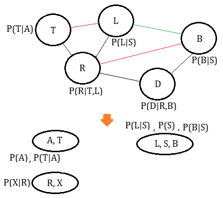 ➄eliminate variable $B$, we get the clique $(R,L,D,B)$, where the green line is the new pairwise connection after $B$ has been removed:
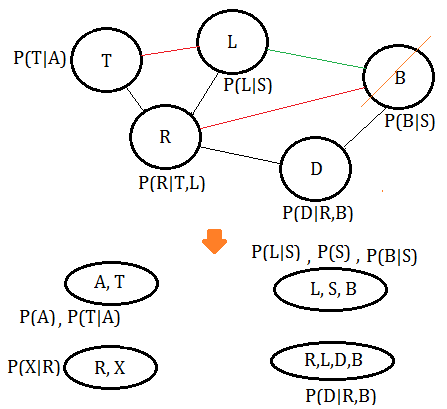 ➅eliminate variable $D$, we get the clique $(R,L,D)$:
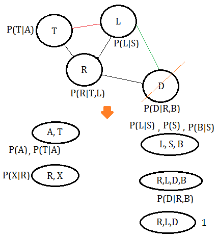 ➆eliminate variable $L$, we get the final clique $(T,L,R)$:
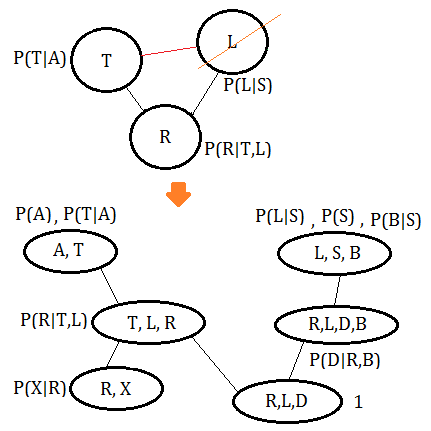 Finally, connect the cliques thus obtained in accordance to the moralized MN(This might not be a perfect clique tree).
[2]
What is $P(L\vert X=y,A=y)$?
Choose $(R,L,D)$ as the pivot:
➀$f_{1}$ and $f_{2}$ are the same:
$f_{1}(T)$=$P(A=y)\cdot P(T\vert A=y)$
$f_{2}(R)$=$P(X=y\vert R)$
➁$f_{3}(L,R)$=$\sum_{T}P(R\vert T,L)\cdot f_{1}(T)\cdot f_{2}(R)$
➂$f_{4}(L,B)$=$\sum_{S}P(S)\cdot P(L\vert S)\cdot P(B\vert S)$
➃$f_{5}(R,D)$=$\sum_{B}P(D\vert R,B)$
➄take $H_{\alpha}(R,L,D)$
=$\sum_{B}f_{3}(L,R)\cdot f_{4}(L,B)\cdot f_{5}(R,D)\cdot 1$ as the joint probability function in this clique tree.
➅compare with the $H(R,L,B)$ in The Bayesian Network Propagation And Clique Tree, we turn $f_{5}(R,D)$ into $f_{5.5}(R,B)$:
$f_{5.5}(R,B)$=$\sum_{D}P(D\vert R,B)$, therefore,
$H_{\alpha}(R,L,D)$
=$\sum_{B}f_{3}(L,R)\cdot f_{4}(L,B)\cdot f_{5}(R,D)\cdot 1$
=$f_{3}(L,R)\cdot f_{4}(L,B)\cdot f_{5.5}(R,B)\cdot 1$
=$H_{\alpha}(R,L,B)$ in this clique tree.
=$H(R,L,B)$ in The Bayesian Network Propagation And Clique Tree
The answer of $P(L\vert X=y,A=y)$ would just be the same!!!
The clique trees are compared in below graph, the new tree is under the original tree:
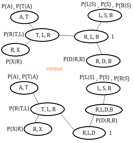 The functions associated with original clique tree are listed below:
$f_{1}(T)$=$P(A=y)\cdot P(T\vert A=y)$
$f_{2}(R)$=$P(X=y\vert R)$
$f_{3}(L,B)$=$\sum_{S}P(S)\cdot P(L\vert S)\cdot P(B\vert S)$
$f_{4}(R,B)$=$\sum_{D}P(D\vert R,B)$
$f_{5}(L,R)$=$\sum_{T}f_{1}(T)\cdot f_{2}(R)\cdot P(R\vert T,L)$
$H(R,L,B)$=$f_{3}(L,B)\cdot f_{4}(R,B)\cdot f_{5}(L,R)\cdot 1$
Very Different Elimination Order Constructed Clique Tree Makes The Same Propagation::by mjtsai1974
In this section, I’d like to prove that by using very different elimination order in clique tree construction process will you get the identical propagation of message passing for the same given BN.
[Question]
Suppose we are give the same above BN, this time, the elimination order is $X,A,T,R,B,D,L,S$, with the clique tree thus constructed, we are asked for the same $P(L\vert X=y,A=y)$, what’s it?
[1]
Clique tree construction
Assume we are give the same above BN, the elimination order is $X,A,T,R,B,D,L,S$, proceed with the following steps:
➀moralize the BN to get the MN.
➁eliminate variable $X$, we get the clique $(X,R)$.
➂eliminate variable $A$, we get the clique $(A,T)$.
➃eliminate variable $T$, we get the clique $(T,L,R)$.
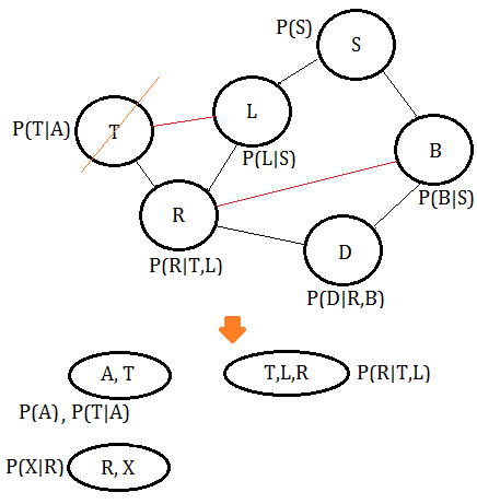 ➄eliminate variable $R$, we get the clique $(R,L,D,B)$.
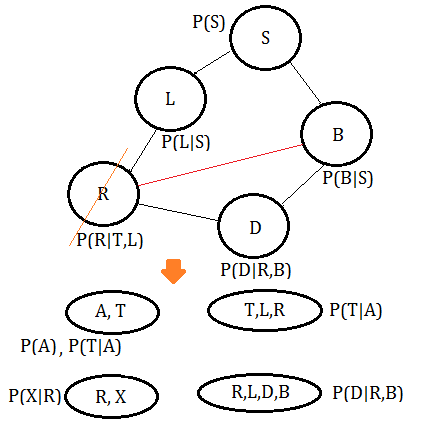 ➅eliminate variable $B$, we get the clique $(B,S,D)$.
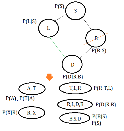 ➆eliminate variable $D$, we get the clique $(L,S,D)$.
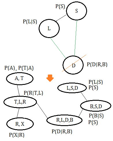 Finally, connect the cliques thus obtained in accordance to the moralized MN(This might not be a perfect clique tree).
[2]
What is $P(L\vert X=y,A=y)$?
Choose $(T,L,R)$ as the pivot:
➀$f_{1}$ and $f_{2}$ are the same:
$f_{1}(T)$=$P(A=y)\cdot P(T\vert A=y)$
$f_{2}(R)$=$P(X=y\vert R)$
➁$f_{3}(L,D)$=$\sum_{S}P(L\vert S)\cdot P(S)$
➂$f_{4}(B,D)$=$\sum_{S}P(B\vert S)\cdot P(S)$
➃$f_{5}(R)$=$\sum_{B,D}P(D\vert R,B)\cdot f_{3}(L,D)\cdot f_{4}(B,D)$
➄take $H_{\beta}(T,L,R)$
=$P(R\vert T,L)\cdot f_{1}(T)$
$\;\;\cdot f_{2}(R)\cdot f_{5}(R)$ as the joint probability function in this clique tree.
➅compare with the $H(R,L,B)$ in The Bayesian Network Propagation And Clique Tree, we turn $f_{5}(R)$ into $f_{5.5}(R,B)$:
$f_{5.5}(R,B)$=$\sum_{D}P(D\vert R,B)\cdot f_{3}(L,D)\cdot f_{4}(B,D)$, therefore,
$H_{\beta}(T,L,R)$
=$P(R\vert T,L)\cdot f_{1}(T)$
$\;\;\cdot f_{2}(R)\cdot f_{5}(R)$
=$\sum_{T}P(R\vert T,L)\cdot f_{1}(T)$
$\;\;\cdot f_{2}(R)\cdot f_{5.5}(R,B)$
=$H_{\beta}(R,L,B)$
=$H(R,L,B)$ in The Bayesian Network Propagation And Clique Tree
The answer of $P(L\vert X=y,A=y)$ would just be the same!!!
The clique trees are compared in below graph, the new tree is under the original tree:
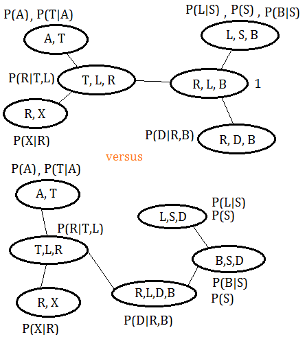 The functions associated with original clique tree could be found in prior section.
The Target: Minimal Clique Trees
A clique tree is minimal if none of its cliques are subsets of their neighbors, the ideal version after variable elimination should be minimal.
Below exhibits different VE leads to different clique trees(non-minimal):
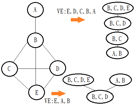 The ideal minimal clique tree would the illustration:
 Current introduced buildCliqueTree() algorithm might not guarantee to have the minimal result, in the incoming future, I might develop a new algorithm for this. (to be conti…)
Clique Tree Is Variable-Connected
The clique tree by buildCliqueTree() from the un-connected MN is variable-connected.
proof::mjtsai1974
By using mathematics induction fashion, we can prove it.
[1]
the case of $1$ clique
Suppose only one clique in the tree, this just holds.
[2]
the case of $n$ cliques
Suppose it holds for $n$ cliques in the tree $\tau’$, next to prove it holds for $n+1$ cliques in the tree $\tau$.
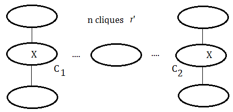 Below is the pre-requisite to next prove step:
➀the tree $\tau’$ contains cliques $C_{1}$ and $C_{2}$ with variable $X$ in it.
➁since $\tau’$ is the clique tree, variable $X$ exists in all the cliques of the path in between $C_{1}$ and $C_{2}$.
[3]
the case of $n+1$ cliques
We’d like to show $X$ exists in all the cliques of the path in between $C_{1}$ and $C_{2}$ in tree of $n+1$ cliques.
To create tree $\tau$, we make below assumption:
➀$C_{1}$ is the clique by removing variable $Z$, where variable $X$ is not $Z$(since $X\in C_{1}\cap C_{2}$), therefore $X\in S$.
➁$\tau’$ is the tree obtained after ➀.
➂suppose $S’$ is obtained by removing some other node in $S$(not $X$), then $S’ \subseteq S$.
➃or suppose $S’$ is obtained by removing some other variables in adjacent to all variables in $S$, then $S’$=$S$.
➄for bothe case $S’ \subseteq S$ or $S’$=$S$, then $X\in S$ and $X\in S’$ must all hold. By taking $\tau$=$C_{1}$+$\tau’$, trivially, the variable exists in the cliques of the path in between $C_{1}$ and $C_{2}$.
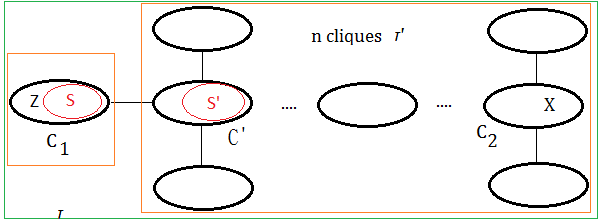
Evenmore, for the condition that keeping ➀,➁ the same, where $S’$ is obtained by removing variable $X$ from $S$, then $S’ \subset S$, that is to say $C’$=$S’\cup X$. By taking $\tau$=$C_{1}$+$\tau’$, we also find it true that the variable exists in the cliques of the path in between $C_{1}$ and $C_{2}$.

Addendum
➀Introduction to Bayesian Networks, Lecture 5: Inference as Message Propagation, Nevin L. Zhang, lzhang@cse.ust.hk, Department of Computer Science and Engineering, Hong Kong University of Science and Technology, Fall 2008
➁Clique Tree Algorithm - Computation
➂Clique Trees, Amr Ahmed, CS CMU, October 23, 2008
➃Graphical Models - Lecture 11: Clique Trees, Andrew McCallum, mccallum@cs.umass.edu
25 Sep 2018
Prologue To The Bayesian Network Propagation And Clique Tree
The introduction of clique tree algorithm aims at posterior belief update distributed in all variables of a network by means of message propagation.
The Clique Tree
A clique tree is an undirected tree, where:
➀each node in the tree is a set of variables, called a clique.
➁if one variable appears in 2 cliques, it must exist in all the cliques in the path between the 2 cliques. It is variable-connected.
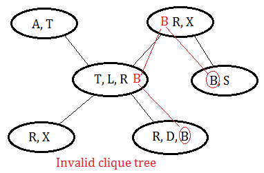 This is an invalid clique tree, variable B should exist in all the cliques in the path in between cliques of $(B,S)$ and $(R,D,B)$.
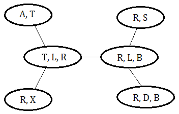 This is a valid clique tree, since it meets the criteria that a variable could be found on all cliques in the path between 2 cliques containing it.
A clique tree covers a Bayesian network if below conditions are meet:
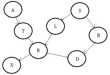 ➀the union of the cliques is the set of the variables in the Bayesian network.
➁for any variable $X$, the clique tree has one clique containing this variable with all its parent variables, such clique is called the family cover clique of $X$.
Suppose we are given above Bayesian network, below clique tree is just one such example.
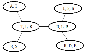
The Clique Tree For Variable Elimination
Supposed we are given this Bayesian network and would like to make the posterior belief update of all variables based on the observed evidence. This paragraph will guide you through the whole process by using the clique tree.
[1]
Initialize the cliques with independence probability distribution of BN variables
For each variable $X$ in Bayesian network:
➀find the probability of $P(X\vert Pa(X))$ and attach it onto the clique containing $X$.
➁if the clique has no probability of independence attached, set it to the identity function.
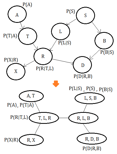 Trivially, the multiplication of all functions on the clique tree is equivalent to the full joint probability distribution in the Bayesian network.
[2]
Instantiate the variable with the observed evidence
Using the same Bayesian network, we denote the observed evidence as $E$, in the real world, we can have observation of multiple variables at the same time.
Suppose we have observed $A=y$ and $X=y$, to instantiate the clique tree, we associate the independence probability function containing $A$ and $X$ with the observed value $y$.
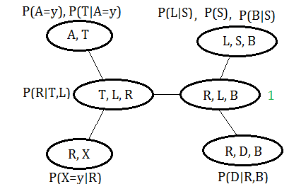 If we take $\chi$ to be all unobserved variables, $P(\chi,E)$ is just the multiplication of all functions on the clique tess, which will laterly be proved.
[3]
Choose pivot for reference
➀for one query variable case, choose the clique containing that variable in it to be the pivot.
Suppose we’d like to query for $P(L\vert A=y,X=y)$, based on the observation of $A=y,X=y$, in the same example, take the clique $(R,L,B)$ to be the pivot, the $(T,L,R)$ could also be the candidate.
➁for case of two query variables, then combine the cliques of the queried variable together as the pivot, or just choose the clique containing these 2 queried variables, if any exists.
Suppose we’d like to query for $P(T,L\vert A=y,X=y)$, we can directly take the clique $(T,L,R)$ as to pivot. If we’d like to query for $P(T,B\vert A=y,X=y)$, then combine the cliques $(T,L,R)$,$(R,L,B)$ just holds.
➂for multiple query variables case, follow ➁’s fashion, could we reach the goal.
[4]
Pass the messages from the leafs to the pivot
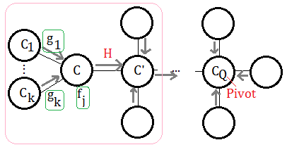
When we have a clique tree constructed, the messages(evidence) are passed from the leafs to the pivot node. Supposed we have such example of undirected graph, the clique is expressed by uppercase C for better understanding.
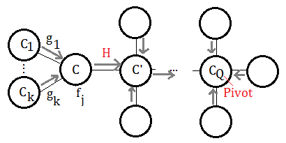 This exhibition reveals the portion mostly closed to the target pivot $C_{Q}$, the messages are coming from $C_{i}$, where $i$=$1$ to $k$, such message passing are triggered by the observed evidence on leaf nodes, maybe far away from these $C_{i}$s.
➀$g_{i}$ is the message from $C_{i}$ to $C$.
➁$f_{j}$ is the function attached to $C$.
➂the messages passed to $C$, are trsnafered to $C’$, we denote it $H$.
$H((C\cap C’)-E)$=$\sum_{C\backslash C’\cup E}\prod_{i}g_{i}\prod_{j}f_{j}$
The summation over elements purely from $C$, not belonging to $C’$ and $E$(evidence).
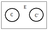 The term $(C\cap C’)-E$ is better understood by this illustration. Since $C$ and $C'$ are independent, the intersection of the 2 nodes is null. It’s the evidence existing in the space in between $C$ and $C'$, after we minus $E$, what we want is the pure message from $C$ to $C'$.
[5]
Posterior belief update
Supposed we’d like to query for $P(Q|E=e)$ in above given graph of clique tree, and we take $H(Q,\chi)$ to be the function attached or send to $C_{Q}$, where $\chi$ stands for all unobserved variables other than $Q$ in $C_{Q}$:
$P(Q|E=e)$=$\frac {\sum_{\chi}H(Q,\chi)}{\sum_{Q,\chi}H(Q,\chi)}$
Posterior Belief Update Illustration In Clique Tree
[Question]
Using the same clique tree, suppose we are given the observed evidence on $A=y$ and $X=y$, we’d like to make inference on $P(L\vert A=y,X=y)$.
[Answer]
Let’s illustrate by this graph, similar to variable elimination process.
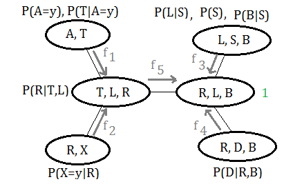 ➀do the join over $A=y$ in clique $(A,T)$:
$f_{1}(T)$=$P(A=y)\cdot P(T\vert A=y)$
➁directly take the only attached function in clique $(R,X)$:
$f_{2}(R)$=$P(X=y\vert R)$
➂do the join over $S$ in clique $(L,S,B)$, we’d like to move toward the pivot:
$f_{3}(L,B)$=$\sum_{S}P(S)\cdot P(L\vert S)\cdot P(B\vert S)$
➃do the join over $D$ in clique $(R,D,B)$, we’d like to move toward the pivot:
$f_{4}(R,B)$=$\sum_{D}P(D\vert R,B)$
➄in clique $(T,L,R)$, collect the message from clique $(A,T)$ and $(R,X)$, pass it to the pivot:
$f_{5}(L,R)$=$\sum_{T}f_{1}(T)\cdot f_{2}(R)\cdot P(R\vert T,L)$
This time, join over $T$.
➅thus we have $f_{3}(L,B)$,$f_{4}(R,B)$ and $f_{5}(L,R)$, the joint probability is thus distributed and expressed as:
$H(R,L,B)$=$f_{3}(L,B)\cdot f_{4}(R,B)\cdot f_{5}(L,R)\cdot 1$
Finally, $P(L\vert A=y,X=y)$=$\frac {\sum_{R,B}H(R,L,B)}{\sum_{R,L,B}H(R,L,B)}$, since $H(R,L,B)$ already encompass $A=y$ and $X=y$ in it.
The Clique Tree Propagation Algorithm: Computation Sharing In All Queries
[1]
The algorithm of two sweep message passing
➀the first sweep is collection, from the leafs to the pivot, above posterior belief update illustration is the example.
➁the second sweep is distribution, from the pivot to the leafs. Next to illustrate it.
[2]
Propagation from the pivot to the leafs
Just like your eyes see somthing, stimulation from certain observation of evidence to the brain, next would be the inspiration from the brain central point back to each distinct parts that had joined in this message frowarding process, finally back to your eyes. This explains why human sometimes tracks object movement, maybe.
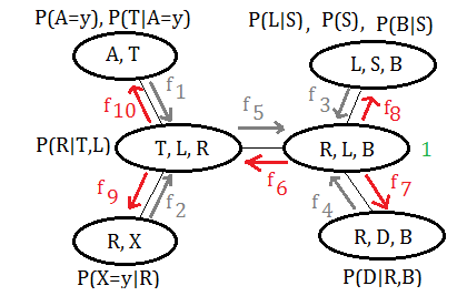 Using the same example of clique tree, the message is distributed from the pivot $(R,L,B)$ to all other cliques in reversed direction.
➀$f_{6}(R,L)$=$\sum_{B}f_{3}(L,B)\cdot f_{4}(R,B)\cdot 1$
Combine the $f_{3}(L,B)$,$f_{4}(R,B)$ by joining over $B$, could we have the function of message passing to clique $(T,L,R)$.
➁$f_{7}(R,B)$=$\sum_{L}f_{3}(L,B)\cdot f_{5}(R,L)\cdot 1$
➂$f_{8}(L,B)$=$\sum_{R}f_{4}(R,B)\cdot f_{5}(R,L)\cdot 1$
➃$f_{9}(R)$=$\sum_{T,L}f_{1}(T)\cdot f_{6}(R,L)\cdot P(R\vert T,L)$
Combine $P(R\vert T,L)$ with $f_{1}(T)$ and $f_{6}(R,L)$, join over $T,L$, could we have such expression of the message passing to clique $(R,X)$ from the pivot.
➃$f_{10}(T)$=$\sum_{R}f_{2}(R)\cdot f_{6}(R,L)$
Have you found that the function of the message from the pivot to the leafs are all expressed in terms of the variables the same as it is in the clique from which passes message to the pivot.
[3]
Posterior belief update after distribution::mjtsai1974
Suppose you’d like to infer $P(L\vert A=y,X=y)$ in $(T,L,R)$, since we have $f_{1}(T)$,$f_{2}(R)$,$f_{6}(R,L)$ send to $(T,L,R)$ and $P(R\vert T,L)$ attached to it:
➀$I(T,L,R)$
=$\sum_{B}f_{1}(T)\cdot f_{2}(R)\cdot$
$\;\;f_{3}(L,B)\cdot f_{4}(R,B)\cdot P(R\vert T,L)$
=$f_{1}(T)\cdot f_{2}(R)\cdot f_{6}(R,L)\cdot P(R\vert T,L)$
, where $f_{6}(R,L)$ is the join of $f_{3}(L,B)$ and $f_{4}(R,B)$ over $B$.
➁$P(L\vert A=y,X=y)$
=$\frac {\sum_{T,L,R}I(T,R)}{\sum_{T,L,R}I(T,L,R)}$
➂by using $H(R,L,B)$ or $I(T,L,R)$ is to calculate $P(L\vert A=y,X=y)$ on the same sets of functions!
This is my explain of computation sharing.
The Clique Tree Properties
[Property 1]
The arguemnts of the functions attached or send to a clique are all veriables in the clique
In mjtsai’s explain:
➀before $C$ sends to $C’$, the arguments of the functions attached to $C$ or send to $C$ would be passed to a clique $C’$ are all variables in the clique $C$.
➁after $C$ sends to $C’$, the arguments of the functions attached to $C$ or send to $C$ has been passed to a clique $C’$ are all variables in the clique $C$.
proof::mjtsai1974
Using the same clique tree in above paragraph, focus on the left pink marked part.
➀by given we have $f_{j}$ attached to $C$ and passing message of $g_{i}$ from $C_{i}$.
➁the function of the messgae from $C$ to $C’$ is thus defined:
$H((C\cap C’)-E)$=$\sum_{C\backslash C’\cup E}\prod_{i}g_{i}\prod_{j}f_{j}$
therefore, the arguments of the functions in the passing messgae from $C$ to $C’$ are all the variables in $C$.
[Property 2]
Product of functions attached to or send to all un-activated cliques=$P(\chi,E=e)$, where $\chi$ stands for all unobserved variables in these un-activated cliques
proof::mjtsai1974
We denote a clique is un-activated if it has not send out messages.
Using the same clique tree in below paragraph.
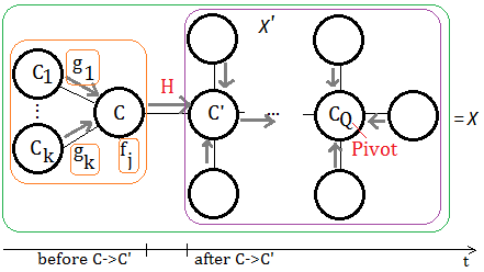 ➀take $\chi$ to be the set of unobserved variables in all un-activated cliques, before $C$ send message to $C’$.
➁take $\chi’$ to be the set of unobserved variables in all un-activated cliques, after $C$ send message to $C’$.
➂take $r$ to be the product of functions attached to or send to all un-activated cliques, after $C$ send message to $C’$, then $r$ is a function of $\chi’$, that is $r(\chi’)$, where $H$ is not included, since $H$ is just the function of message passing in between!!
➃consider the message passing from $C$ to $C’$, take $C\backslash C’\cup E$ into account, for simplicity, treat $Z$=$C\backslash C’\cup E$, where $Z\in C$ and $Z\not\in C’$ is of no doubt.
 ➄under ➃, we have $\chi$=$Z\cup\chi'$, the full illustration is exhibited below:
 ➅suppose property 2 is true that
$r(\chi’)\cdot\prod_{i}g_{i}\prod_{j}f_{j}$=$P(\chi,E=e)$, next, consider the time point of "before being after"(by $H$) and "being after"(by $r(\chi’)$) $C$ send messages to $C’$, the combinatory of these two distributions provides a full image of distribution in this cliquer tree for the whole "after" $C$ send messages to $C'$:
$r(\chi’)\cdot H((C\cap C’)-E)$
=$r(\chi’)\cdot\sum_{C\backslash C’\cup E}\prod_{i}g_{i}\prod_{j}f_{j}$
=$\sum_{Z}r(\chi’)\cdot\prod_{i}g_{i}\prod_{j}f_{j}$
=$\sum_{Z}P(\chi,E=e)$
=$\sum_{Z}P(Z,\chi’,E=e)$
=$P(\chi’,E=e)$
➆$r(\chi’)\cdot\prod_{i}g_{i}\prod_{j}f_{j}$=$P(\chi,E=e)$
$\Leftrightarrow$
$r(\chi’)\cdot H((C\cap C’)-E)$=$P(\chi’,E=e)$
That is to say before $C$ send messages to $C'$, the product of all functions attached to or send to all un-activated cliques(at this moment, $C$, $C'$ and others are all un-activated) and after $C$ send messages to $C'$, the the product of all functions attached to or send to all un-activated cliques(at this moment, $C'$ and others are all un-activated) are all equivalent to:
$P(Unobserved\;vars,E=e)$…by mjtsai1974.
Addendum
➀Introduction to Bayesian Networks, Lecture 5: Inference as Message Propagation, Nevin L. Zhang, lzhang@cse.ust.hk, Department of Computer Science and Engineering, Hong Kong University of Science and Technology, Fall 2008
26 Aug 2018
Prologue To Propagation In The Bayesian Network
The respective and retrospective inferences ascertained by means of variable elimination is also computation expensive, it works for one variable at a time, the same operation would be repeated upon new inference on other variables is requested.
An alternative to overcome these limitations is by using propagation in the Bayesian network.
Posterior Probability(Belief) Update Upon New Evidence Arrives
[1]
Posterior probability(belief)
The posterior probability(belief) of a random variable $X$=$x$, given evidence $E$=$e$, is expressed as $Bel(x)\overset\triangle=P(x\vert e)$. The evidence could be further classified as 2 distinct subsets:
➀$e_{X}^{-}$ denotes the evidence introduced through its children nodes.
➁$e_{X}^{+}$ stands for the evidence coming from its parent nodes, for $X$ to be a root node, $e_{X}^{+}$ is the background.
[2]
Deduction of $Bel(x)$
Assume $e_{X}^{-}$ and $e_{X}^{+}$ are independent, then the belief of $X$=$x$:
$Bel(x)$
=$P(x\vert e_{X}^{-},e_{X}^{+})$
=$\frac {P(e_{X}^{-},x\vert e_{X}^{+})}{P(e_{X}^{-}\vert e_{X}^{+})}$
=$\frac {P(e_{X}^{-}\vert x,e_{X}^{+})\cdot P(x\vert e_{X}^{+})}{P(e_{X}^{-}\vert e_{X}^{+})}$
=$\frac {P(e_{X}^{-}\vert x)\cdot P(x\vert e_{X}^{+})}{P(e_{X}^{-})}$
Why we have such deduction?
➀the evidence $e_{X}^{-}$ is given by hypothesis $X$=$x$, and the background context $e_{X}^{+}$, that explains $P(e_{X}^{-}\vert x,e_{X}^{+})$.
➁$P(x\vert e_{X}^{+})$ says that the hypothesis $X$=$x$ is propagated from the background context $e_{X}^{+}$.
➂the normalizing factor $P(e_{X}^{-}\vert e_{X}^{+})$ encompasses everything ranging from the background context to the final observed evidence, since $e_{X}^{-}$ and $e_{X}^{+}$ are independent, the denominator part becomes $P(e_{X}^{-})$.
$P(e_{X}^{-})$
=$P(e_{X}^{-}\vert e_{X}^{+})$
=$P(e_{X}^{-}\vert x,e_{X}^{+})\cdot P(x\vert e_{X}^{+})$
=$P(e_{X}^{-}\vert x)\cdot P(x\vert e_{X}^{+})$
=$\lambda(X)\cdot\pi(X)$
[3]
Generalization of $Bel(x)$
Most of the textbooks have below common definition:
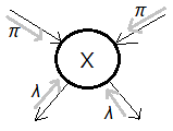
➀$\pi(x)$=$P(x\vert e_{X}^{+})$ is the respective(predictive) direction of propagation.
➁$\lambda(x)$=$P(e_{X}^{-}\vert x)$ is retrospective(diagnostic) direction of propagation.
We thus express the belief of $x$ as $Bel(x)$=$\alpha\cdot\pi(x)\cdot\lambda(x)$,
where $\alpha$ is the normalizing constant, in this illustration,
$\alpha$
=$[P(e_{X}^{-})]^{-1}$
=$[\sum_{x}\pi(x)\cdot\lambda(x)]^{-1}$
[4]
Message passing is propagation
New evidence enters a network when a variable is instantiated, ie when it receives a new value from the outside world. When this happens, the posterior probability of each node in the whole network must be re-calculated.
This is achieved by message passing, known as progapation.
Propagation Illustration In Causal Tree
Given a causal tree of this serial chain Bayesian network, where $\lambda(Y)$=$P(e_{Y}^{-}\vert Y)$.

[1]
Forward propagation
➀$W$ is now the root node, the background context is the only forward propagated evidence.
$\pi(w)$=$P(w\vert e_{W}^{+})$=$P(w)$, for $w\in W$.
➁for node $X$, it receives the forward propagated evidence pass through it, thus:
$\pi(x)$
=$P(x\vert e_{X}^{+})$
=$P(x\vert e_{WX}^{+})$
=$\sum_{w}P(x\vert w)\cdot P(w\vert e_{W}^{+})$, for $w\in W$.
$\Rightarrow\pi(X)$=$P(X\vert W)\cdot\pi(W)$
Node $X$ receives $W$ forward propagated evidence $P(w\vert e_{W}^{+})$, with each $X=x$ weighted by $P(x\vert w)$ for all $w\in W$.
➂similarly, $\pi(Y)$=$P(Y\vert X)\cdot\pi(X)$
[2]
Backward propagation
➀$Y$ is the leaf node, the evidence of observation is the only backward propagated message.
$\lambda(y)$=$P(e_{Y}^{-}\vert y)$
➁as $X$ receives the backward propagated evidence from $Y$, then:
$\lambda(x)$
=$P(e_{X}^{-}\vert x)$
=$P(e_{XY}^{-}\vert x)$
=$\sum_{y}P(y\vert x)\cdot\lambda(y)$, for $y\in Y$.
$\Rightarrow\lambda(X)$=$P(Y\vert X)\cdot\lambda(Y)$
For each $x\in X$, $\lambda(x)$ is weighted by $P(y\vert x)$ with $\lambda(y)$, for all $y\in Y$.
➁similarly, for node $W$,
$\lambda(w)$
=$P(e_{W}^{-}\vert w)$
=$P(e_{WX}^{-}\vert w)$
=$\sum_{x}P(x\vert w)\cdot\lambda(x)$
$\Rightarrow\lambda(W)$=$P(X\vert W)\cdot\lambda(X)$
Propagation Illustration In Multiple Child Nodes
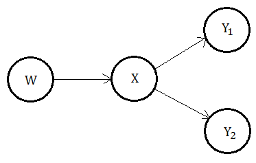
Now take a look at the illustration for the case of multiple child nodes.
[1]
Backward propagation
This time, we begin by inspecting the behavior in $\lambda$. We have evidence on the subtree at node $X$ partitioned into 2 disjoint sets $e_{XY_{1}}^{-}$,$e_{XY_{2}}^{-}$.
➀as $X$ receives backward propagated evidence from $Y_{1}$, $Y_{2}$, the backward propagation is in joint distribution form:
$\lambda(x)$…$x\in X$
=$P(e_{X}^{-}\vert x)$
=$P(e_{XY_{1}}^{-}\vert x)\cdot P(e_{XY_{2}}^{-}\vert x)$
=$\prod_{Y_{i}\in Y}P(e_{XY_{i}}^{-}\vert x)$…multiple $Y_{i}$ children
$\Rightarrow\lambda(x)$=$\lambda_{Y_{1}}(x)\cdot\lambda_{Y_{2}}(x)$
➁as $X$ backward propagates the evidence to $W$:
$\lambda(w)$…$w\in W$
=$\sum_{x}P(x\vert w)\cdot\lambda(x)$
$\Rightarrow\lambda_{X}(W)$=$P(X\vert W)\cdot\lambda(X)$
[2]
Forwardward propagation
➀as to the forward propagated evidence in node $X$, that’s $\pi(X)$, we evaluate it from its parent node $W$.
$\pi(x)$…$x\in X$
=$P(x\vert e_{X}^{+})$
=$P(x\vert e_{WX}^{+})$
=$\sum_{w}P(x\vert w)\cdot\pi(w)$
$\Rightarrow\pi(X)$=$P(X\vert W)\cdot\pi(W)$
[3]
Forwardward propagation to multiple descendent
The forward propagated evidence in node $X$ would be taken into 2 distinct parts. Consider the evidence forward propagated from $X$ to $Y_{1}$, it consists of 2 major factors:
➀the forward propagated evidence from $W$.
➁the backward propagated evidence from $Y_{2}$.
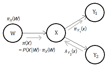 The point is that the total forward propoagated evidence from $X$ to $Y_{2}$ is the joint probability function in combinatory format of these 2 factors.
$\pi_{Y_{1}}(x)$
=$P(x\vert e_{X}^{+},e_{Y_{2}}^{-})$
=$\frac {P(e_{Y_{2}}^{-}\vert x,e_{X}^{+})\cdot P(x\vert e_{X}^{+})}{P(e_{Y_{2}}^{-}\vert e_{X}^{+})}$
=$\frac {P(e_{Y_{2}}^{-}\vert x)\cdot P(x\vert e_{X}^{+})}{P(e_{Y_{2}}^{-}\vert e_{X}^{+})}$
, where $x\in X$ and $e_{Y_{2}}^{-}\in e_{X}^{-}$, more precisely, we can take $e_{Y_{2}}^{-}$=$e_{XY_ {2}}^{-}$, next to expand it.
[4]
Forwardward propagation to multiple descendent: extension
proof::mjtsai1974
Continue from $\pi_{Y_{1}}(x)$:
➀multiply nominator and denominator by $P(e_{Y_{1}}^{-}\vert x)$:
$\pi_{Y_{1}}(x)$
=$\frac {P(e_{Y_{2}}^{-}\vert x)\cdot P(x\vert e_{X}^{+})\cdot P(e_{Y_{1}}^{-}\vert x)}{P(e_{Y_{2}}^{-}\vert e_{X}^{+})\cdot P(e_{Y_{1}}^{-}\vert x)}$
➁$P(e_{Y_{2}}^{-}\vert e_{X}^{+})$
=$\sum_{x}P(e_{Y_{2}}^{-}\vert x,e_{X}^{+})\cdot P(x\vert e_{X}^{+})$
=$\sum_{x}P(e_{Y_{2}}^{-}\vert x)\cdot P(x\vert e_{X}^{+})$
=$\alpha_{XY_{2}}^{-1}$
=$P(e_{XY_{2}}^{-})$…$e_{Y_{2}}^{-}$ and $e_{X}^{+}$ are independent
➂we also have further deduction below for $P(e_{X}^{-})$:
$P(e_{Y_{2}}^{-}\vert e_{X}^{+})\cdot P(e_{Y_{1}}^{-}\vert x)$
=$\sum_{x}P(e_{Y_{2}}^{-}\vert x)\cdot P(x\vert e_{X}^{+})\cdot P(e_{Y_{1}}^{-}\vert x)$
=$P(e_{X}^{-})$
=$\alpha_{X}^{-1}$
➃therefore, rewrite ➀:
$\pi_{Y_{1}}(x)$
=$P(x\vert e_{X}^{+},e_{Y_{2}}^{-})$
=$\frac {P(e_{Y_{2}}^{-}\vert x)\cdot P(x\vert e_{X}^{+})\cdot P(e_{Y_{1}}^{-}\vert x)}{P(e_{XY_{2}}^{-})\cdot P(e_{Y_{1}}^{-}\vert x)}$
=$\frac {P(e_{Y_{2}}^{-}\vert x)\cdot P(x\vert e_{X}^{+})\cdot P(e_{Y_{1}}^{-}\vert x)}{\alpha_{XY_{2}}^{-1}\cdot P(e_{Y_{1}}^{-}\vert x)}$
=$\frac {\alpha_{XY_{2}}\cdot P(e_{Y_{2}}^{-}\vert x)\cdot P(x\vert e_{X}^{+})\cdot P(e_{Y_{1}}^{-}\vert x)}{P(e_{Y_{1}}^{-}\vert x)}$
=$\frac {Bel_{Y_{1}}(x)}{\lambda_{Y_{1}}(x)}$
Here, we take $Bel_{Y_{1}}(x)$
=$\alpha_{XY_{2}}\cdot P(e_{Y_{2}}^{-}\vert x)\cdot P(x\vert e_{X}^{+})\cdot P(e_{Y_{1}}^{-}\vert x)$
[5]
Forwardward propagation to multiple descendent: generalization
Given that node $X$ has $n$ multiple child nodes $\{Y_{1},…,Y_{n}\}$, then, the forward propagated evidence from $X$ to $Y_{k}$ could be generalized in below expression:
$\pi_{Y_{k}}(x)$
=$\frac {Bel_{Y_{k}}(x)}{\lambda_{Y_{k}}(x)}$
, where $Bel_{Y_{k}}(x)$=$\alpha_{XY_{k}}\cdot\prod_{i\neq k} P(e_{Y_{i}}^{-}\vert x)\cdot P(x\vert e_{X}^{+})$
Propagation Illustration In Multiple Parent Nodes
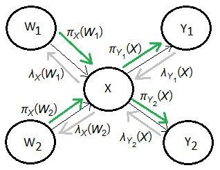
Causal polytree is the structure to be used in this section, each node might have multiple parents.
[1]
Forward propagation
➀the predictive support at $X$ comes from its 2 parents $W_{1}$, $W_{2}$.
$\pi(x)$…$x\in X$
=$P(x\vert e_{X}^{+})$
=$P(x\vert e_{W_{1}X}^{+},e_{W_{2}X}^{+})\cdot P(x\vert W_{1},W_{2})$
=$P(x\vert e_{W_{1}X}^{+})\cdot P(x\vert e_{W_{2}X}^{+})\cdot P(x\vert W_{1},W_{2})$
=$\sum_{w_{1}}\sum_{w_{2}}P(x\vert e_{W_{1}X}^{+})\cdot P(x\vert e_{W_{2}X}^{+})\cdot P(x\vert w_{1},w_{2})$
=$\sum_{w_{1}}\sum_{w_{2}}\pi_{W_{1}}(x)\cdot\pi_{W_{2}}(x)\cdot P(x\vert w_{1},w_{2})$
➁the generalization of forward propagation at $X$ for $n$ parents:
$\pi(x)$=$\sum_{w_{1},…,w_{n}}\pi_{W_{1}}(x)\cdots\pi_{W_{n}}(x)\cdot P(x\vert w_{1},…,w_{n})$
➂as the forward propagation from $X$ to one of its child, say $Y_{k}$, it will have to combine the forward propagation thus obtain above with the backward propagated evidence from $\{Y_{1},…,Y_{k-1},Y_{k+1},…,,Y_{m}\}$, suppose $X$ has $m$ multiple child nodes.
[2]
Backward propagation
➀the diagnostic support at $X$ comes from its 2 children $Y_{1}$, $Y_{2}$, where $\lambda(x)$=$\lambda_{Y_{1}}(x)\cdot\lambda_{Y_{2}}(x)$, must be splitted into 2 parts to be transfered to $W_{1}$, $W_{2}$, which are $\lambda_{X}(w_{1})$,$\lambda_{X}(w_{2})$.
➁to diagnose in $W_{1}$ the symptom/evidence backward propagated from $X$:
$\lambda_{X}(w_{1})$
=$P(e_{W_{1}X}^{-}\vert W_{1})$
=$P(e_{X}^{-},e_{W_{2}X}^{+}\vert W_{1})$
=$P(e_{X}^{-}\vert W_{1})\cdot P(e_{W_{2}X}^{+}\vert W_{1})$
=$P(e_{X}^{-}\vert x)\cdot P(x\vert W_{1})\cdot P(e_{W_{2}X}^{+})$
=$P(e_{X}^{-}\vert x)\cdot P(x\vert W_{1},W_{2})\cdot S_{1}\cdot P(e_{W_{2}X}^{+})$
=$P(e_{X}^{-}\vert x)\cdot P(x\vert W_{1},W_{2})\cdot S_{2}\cdot P(W_{2}\vert e_{W_{2}X}^{+})$
=$P(e_{X}^{-}\vert x)\cdot P(x\vert W_{1},W_{2})\cdot\beta\cdot P(e_{W_{2}X}^{+}\vert W_{2})$
=$\beta\sum_{x}\lambda(x)\cdot\sum_{w_{2}}P(x\vert w_{1},w_{2})\cdot\pi_{W_{2}}(x)$
, where the $S_{1}$,$S_{2}$,$\beta$ are arbitrary constants to hold the equality. We turn from $P(W_{2}\vert e_{W_{2}X}^{+})$ to $P(e_{W_{2}X}^{+}\vert W_{2})$ to express the deduction in terms of $\pi_{W_{2}}(x)$ for its simplicity.
➂the generalization of $n$ multiple parents:
$\lambda_{X}(w_{i})$
=$\beta\sum_{x}\lambda(x)$
$\;\;\cdot\sum_{w_{k}:k\neq i}P(x\vert w_{1},…,w_{n})$
$\;\;\cdot\prod_{k=1:k\neq i}^{n}\pi_{W_{k}}(x)$
[Cautions]
The belief updated by propagation would result in expensive computation consumption when there exists multiple parents. The introduction of propagation aims to eliminate the potential expensive computation of NP-hard order in variable elimination, now it seems that it is struggling over. Next to see the clique tree series, to be believed workable in a lot references.
Addendum
➀A T utorial on Bayesian Belief Networks, Mark L Krieg, Surveillance Systems Division Electronics and Surveillance Research Laboratory, DSTO-TN-0403
➁Lecture 4: Probability Propagation in Singly Connected Bayesian Networks, Duncan Fyfe Gillies, Department of Computing Imperial College London
29 Jul 2018
Prologue To Variable Elimination Order And Moral Graph
The Bayesian network is a DAG(directed acyclic graph), while the moral graph is an undirected version, also known as the Markov network.
The moral graph could facilitate the explanation of the factorization in variable elimination process and its order.
Moral Graph Of A BN(Bayesian Network)
[The moralization algorithm]
➀drop the connectivity in the original Bayesian network, that is to remove the arrow from the arc.
➁connect the parents that shares a common child, that is to marry them.
The resulting undirected graph is the moral graph of a Bayesian network.
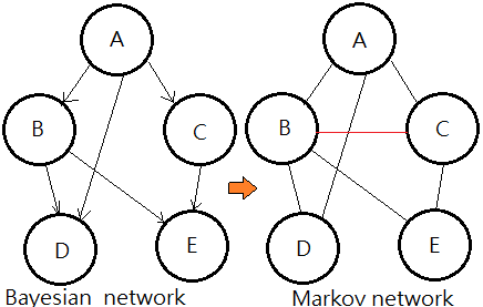
This undirected graph is also named Markov network.
 The Markov network encodes the CPD in the Bayesian network as a factor of all related variables, like $P(E\vert B,C)$ is expressed in a factor form, $f(B,C,E)$, related variables in each distinct CDP are now be connected by an edge.
[Question]
Why we turn the CDP in the Bayesian network into the factorized form in the Markov network?
[Answer]
Because the moral graph is undirected, it is not in conditionally distributed, rather than, in joint distributed!!
I-Map(Independence Map)
[Definition]
Given below 2 prerequisites:
➀let $I(G)$ be the set of all conditional independences implied by the DAG, said $G$.
➁let $I(P)$ be the set of all conditional independences that holds for or belongs to the joint probability distributiuon, said $P$.
We define the DAG $G$ is an I-Map of a distribution $P$, if $I(G)\subseteq I(P)$.
[Full connected DAG]
A fully connected DAG $G$ is an I-Map for any probability distribution, since:
$I(G)$=$\varnothing\subseteq I(P)$ for all $P$
[Minimal I-Map]
$G$ is a minimal I-Map for P, if any removal of a single edge makes it not an I-Map.
➀a joint probability distributrion might have multiple minimal I-Maps.
➁each corresponds to a specific node-ordering.
[Perfect map]
For $I(G)$=$I(P)$, we say $G$ is a perfect map for $P$.
This section could be found at Probabilistic graphical models, David Sontag, New York University, Lecture 2, February 2, 2012, p.5
Concept Of Potentials
[1]
What is a potential?
A potential $\phi_{\chi}$ over a set of random variables $\chi$ is a function that maps each combination of configurations to a non-negative real number.
The conditional probability distribution, joint probability distribution are all the special cases of potential. The domain of a potential $\chi$ is denoted as:
$dom(\phi_{\chi})$=$\chi$
[2]
Moralizing and domain graph
Let $\phi$=$\{\phi_{1},\phi_{2},…,\phi_{n}\}$ to be the potentials over a set of random variables, $\chi$=$\{X_{1},…,X_{m}\}$, and with its domain distributed as $dim(\phi_{i})$=$D_{i}$.
➀the domain graph for $\phi$ is the undirected graph with random variables $X_{1}$,…,$X_{m}$ as nodes and link exists between node pairs belonging to the same domain.
➁it is also known as moral graph.
[3]
Potential and its domain
Given that $\phi$=$\{\phi_{1},…,\phi_{5}\}$ is a set of potentials over $\{X_{1},…,X_{5}\}$, below graph exhibits the potential with respect to its domain:
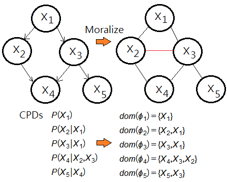 , where $\phi_{1}$=$P(X_{1})$,$\phi_{2}$=$P(X_{2}\vert X_{1})$,$\phi_{3}$=$P(X_{3}\vert X_{1})$,$\phi_{4}$=$P(X_{4}\vert X_{2},X_{3})$,$\phi_{5}$=$P(X_{5}\vert X_{4})$.
[4]
The fill-ins
In variable elimination process, the removal of one variable would possibly generate a new potential over a domain that didn't exist in the original domain graph, such new potential is the fill-in.
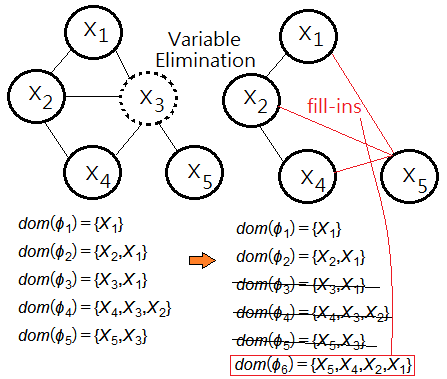 The goal of the most optimal variable elimination sequence is to introduce no extra fill-ins.
Factorization In MN(Markov Network)
[1]
The full/joint PDF in MN
Given below MN, base on our concept that potential is a CPD or a factor of joint distribution, then:
➀$P(A,B,C,D)$…joint PDF
=$\frac {1}{Z}\cdot\phi_{1}(A,B)\cdot\phi_{2}(B,C)\cdot\phi_{3}(C,D)\cdot\phi_{4}(D,A)$
➁Z..normalization factor
=$\sum_{A,B,C,D}\phi_{1}(A,B)\cdot\phi_{2}(B,C)\cdot\phi_{3}(C,D)\cdot\phi_{4}(D,A)$
also called the partition function.
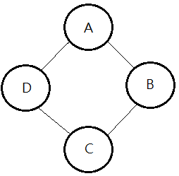
[2]
Tight relation between factorization and independence
$X\perp Y\vert Z$ iff $P(X,Y,Z)$=$\phi_{1}(X,Z)\cdot\phi_{2}(Y,Z)$,
then, $(A\perp C\vert D,B)$ and $(B\perp D\vert A,C)$.
proof::mjtsai1974
To show $(A\perp C\vert D,B)$’s independence:
➀$P(A,C,D,B)$=$\psi_{1}(A,D,B)\cdot\psi_{2}(C,D,B)$
, where $\psi_{i}$ is the potential.
➁for $\psi_{1}(A,D,B)$’s independence:
$B\perp D\vert A$
$\Leftrightarrow P(B,D,A)$=$\phi_{1}(B,A)\cdot\phi_{4}(D,A)$
➂for $\psi_{2}(C,D,B)$’s independence:
$B\perp D\vert C$
$\Leftrightarrow P(B,D,C)$=$\phi_{2}(B,C)\cdot\phi_{3}(D,C)$
➃$P(A,C,D,B)$
=$\phi_{1}(B,A)\cdot\phi_{2}(B,C)\cdot\phi_{3}(D,C)\cdot\phi_{4}(D,A)$
$(B\perp D\vert A,C)$’s independence could be proved in similar way.
[3]
Factors in MN
A factor can below representations:
➀a joint distribution over $D$ by defining $\phi(D)$.
➁a CPD $P(X\vert D)$, by defining $\phi(X\cup D)$
Factors in MN is a more symmetric parameterization that captures the affinities in between related random variables.
The Gibbs Distribution For BN Versus MN
[1]
The Gibbs distribution
A distribution $P_{\phi}$ is a Gibbs distribution if it parameterizes a set of factors $\phi(D_{1})$,…,$\phi(D_{m})$ in the expression:
$\;\;P_{\phi}(X_{1},…,X_{n})$=$\frac {1}{Z}\cdot\phi(D_{1})\cdot\cdots\cdot\phi(D_{m})$, where:
➀$X_{1},…,X_{n}$ are the random variables, $\phi(D_{1}),…,\phi(D_{m})$ are the factors over domains grouped by the related variables and $D_{i}$’s are the domains.
➁$Z$…partition function
=$\sum_{X_{1},…,X_{n}}\phi(D_{1})\cdot\cdots\cdot\phi(D_{m})$
➂a factor is one contribution on the joint operation in variable elimination process.
➃a distribution $P_{\phi}$ with $\phi(D_{1})$,...,$\phi(D_{m})$ factorizes a Markov network if each $\phi_{i}$ is a complete subgraph of it.
[2]
The independence in MN
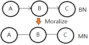 Given this network, we’d like to prove $A\perp C\vert B$ given $P(A,B,C)$=$\frac {1}{Z}\cdot\phi_{A,B}(A,B)\cdot\phi_{B,C}(B,C)$:
proof::mjtsai1974
➀$P(a\vert c)$
=$\frac {P(a\cap c)}{P(c)}$
=$\frac {\sum_{b}P(a,b,c)}{\sum_{a,b}P(a,b,c)}$
=$\frac {\sum_{b}\phi_{A,B}(a,b)\cdot\phi_{B,C}(b,c)}{\sum_{a,b}\phi_{A,B}(a,b)\cdot\phi_{B,C}(b,c)}$
=$\frac {\phi_{A,C}(a,c)}{\phi_{C}(c)}$
It is evident $A$ is independent from $C$ and could be figured out by factors of $A$ and $C$.
➁$P(a\vert b)$
=$\frac {\sum_{c}P(a,b,c)}{\sum_{a,c}P(a,b,c)}$
=$\frac {\sum_{c}\phi_{A,B}(a,b)\cdot\phi_{B,C}(b,c)}{\sum_{a,c}\phi_{A,B}(a,b)\cdot\phi_{B,C}(b,c)}$
=$\frac {\phi_{A,B}(a,b)\cdot\sum_{c}\phi_{B,C}(b,c)}{\sum_{a}\phi_{A,B}(a,b)\cdot\sum_{c}\phi_{B,C}(b,c)}$
=$\frac {\phi_{A,B}(a,b)}{\sum_{a}\phi_{A,B}(a,b)}$
It is evident that the relationship of $A$ and $B$ is estimated by only factor of $A$ and $B$.
➂$P(a,c\vert b)$
=$\frac {P(a,b,c)}{P(b)}$
=$\frac {\phi_{A,B}(a,b)\cdot\phi_{B,C}(b,c)}{\sum_{a,c}\phi_{A,B}(a,b)\cdot\phi_{B,C}(b,c)}$
=$\frac {\phi_{A,B}(a,b)\cdot\phi_{B,C}(b,c)}{\sum_{a}\phi_{A,B}(a,b)\cdot\sum_{c}\phi_{B,C}(b,c)}$
=$\frac {\phi_{A,B}(a,b)}{\sum_{a}\phi_{A,B}(a,b)}\cdot\frac {\phi_{B,C}(b,c)}{\sum_{c}\phi_{B,C}(b,c)}$
=$P(a\vert b)\cdot P(c\vert b)$
This evidence is more confident in our deduction result!! By ➀, ➁, we can conclude that the probability of a variable conditioned on its Markov blanket depends only on potentials involving that node.
[3]
BN with evidence is Gibbs in MN
➀suppose you are given a Bayesian network over $\chi$=$\{A,B,C,D,E\}$ illustrated in this graph, where we have the full joint PDF as:
$P_{\chi}(A,B,C,D,E)$
=$P(E\vert C)\cdot P(D\vert B,C)$
$\;\;\cdot P(B\vert A)\cdot P(C\vert A)\cdot P(A)$
➁given the observation of $e$ on node $E$, then:
$P(a,b,c,d\vert E=e)$
=$\frac {P(a\cap b\cap c\cap d\cap e)}{P(e)}$
=$\frac {P(e\vert c)\cdot P(d\vert b,c)\cdot P(b\vert a)\cdot P(c\vert a)\cdot P(a)}{\sum_{A,B,C,D}P(A,B,C,D,e)}$
Evidently, this is a Gibbs distribution!!
➂we moralize the BN by connecting nodes $B$ and $C$ for they are parents of node $D$, and we have potentials thus expressed:
$\phi_{\chi}(A,B,C,D,E)$
=$\frac {\phi_{A,B,C}(A,B,C)\cdot\phi_{B,C,D}(B,C,D)\cdot\phi_{C,E}(C,E)}{\sum_{A,B,C,D,E}\phi_{A,B,C}(A,B,C)\cdot\phi_{B,C,D}(B,C,D)\cdot\phi_{C,E}(C,E)}$
, where $\phi_{A,B,C}(A,B,C)$=$\phi_{A,B}(A,B)\cdot\phi_{A,C}(A,C)\cdot\phi_{A}(A)$
➃given the observation of $e$ on node $E$, then:
$\phi(a,b,c,d\vert e)$
=$\frac {\phi_{\chi}(a,b,c,d,e)}{\phi(e)}$
=$\frac {\phi_{A,B,C}(a,b,c)\cdot\phi_{B,C,D}(b,c,d)\cdot\phi_{C,E}(c,e)}{\sum_{A,B,C,D}\phi_{A,B,C}(A,B,C)\cdot\phi_{B,C,D}(B,C,D)\cdot\phi_{C,E}(C,e)}$
Surprisingly, a Gibbs distribution again!!
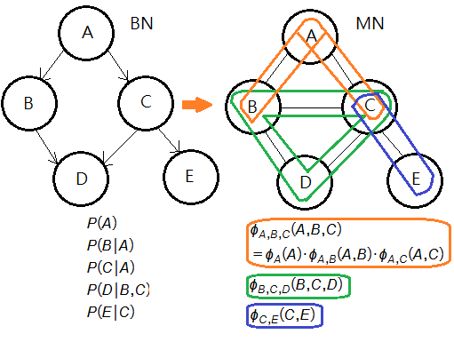 We can conclude that any BN conditioned on evidence can be regarded as a Markov network.
Variable Elimination From BN To MN
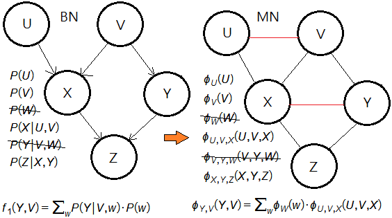
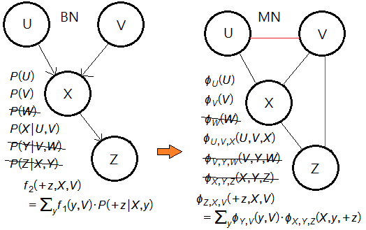
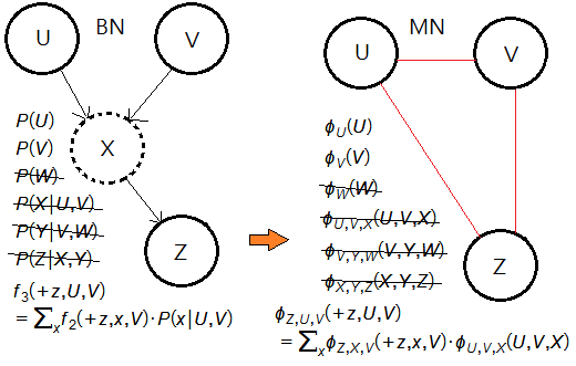
Still using the same example in Prof. Abbeel, steps through a few variable examples for the illustration with a mapping of each step from BN to MN.
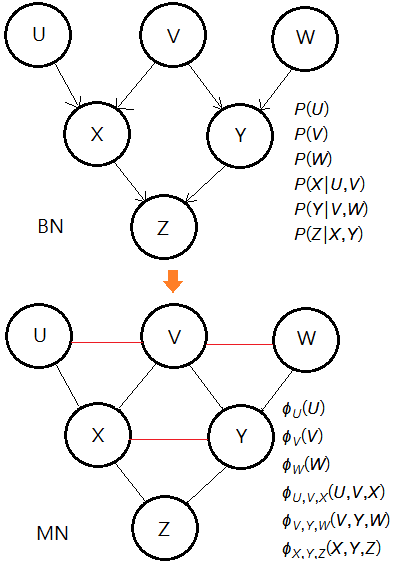 To speed up the path to $P(U\vert +z)$, I use the optimal order of elimination: $W$,$Y$,$X$,$V$
➀eliminate the node $W$.
 ➁eliminate the node $Y$.
 ➂eliminate the node $X$.
 ➃eliminate the node $V$.
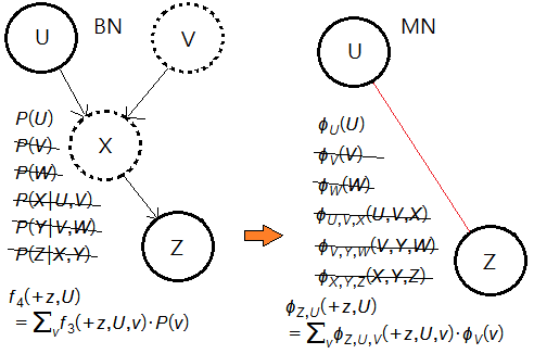 ➄therefore, we have:
$P(U\vert +z)$
=$\frac {f_{4}(+z,U)\cdot P(U)}{\sum_{u}f_{4}(+z,u)}$
=$\frac {\phi_{Z,U}(+z,U)\cdot\phi_{U}(U)}{\sum_{u}\phi_{Z,U}(+z,u)}$
We conclude that each elimination in BN could be well expressed in terms of potentials in MN.
Addendum
➀Variable elimination, CS228, Stefano Ermon
➁Probabilistic graphical models, David Sontag, New York University, Lecture 2, February 2, 2012
➂Bayesian networks and decision graphs, F.V.Jensen, Springer-Verlag New York, 2001
➃Probabilistic graphical models, Raquel Urtasun and Tamir Hazan, TTI Chicago, April 4, 2011
➄From Bayesian networks to Markov networks, Sargur Srihari
15 Jul 2018
Prologue To Variable Elimination In Bayesian Network
Inference via Bayesian network could be achieved by probabilistic marginalization, i.e. summing out over irrelevant or hidden variables.
Inference Via Bayesian Network
Given a well-constructed BN of nodes, 2 types of inference are supported:
➀predictive support(top-down reasoning) with the evidence nodes connected to node $X$, through its parent nodes, the same direction as predictive propagation.
➁diagnostic support(bottom-up reasoning), with vidence nodes connected to node $X$, through its children nodes, the same direction as retrospective propagation.
In my Bayesian articles, I have guided you through both types of support by means of variable enumeration over the factorized terms of full joint PDF(probability distribution function). Most of the examples are all in small network, trivially, variable enumeration is old, she will hold for complex model consisting of a lot random variables, resulting in high expenditure of computation efficiency. Therefore, another technique of variable elimination is introduced.
Example: Illustration Of Variable Elimination
This example is simplified from variable elimination, Peter Norvig.
[Question]
Suppose you are using a Bayesian network to infer the relationship in between raining, traffic and late(to office). The probability of raining and the conditional probability of traffic jam, given raining, and being late, given traffic jam are all depicted in this graph. What’s the probability of being late?
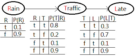
[Answer]
This is to ask for $P(L=t)$. The full joint PDF would be $P(R,T,L)$=$P(L\vert T)\cdot P(T\vert R)\cdot P(R)$.
By the old variable enumeration, $P(L=t)$=$\sum_{R}\sum_{T}P(R,T,L=t)$, the nested summation over $T$ would be proceeded inside the outer summation over $R$. Here, we’d like to further reduce the computation complexity by means of variable elimination.
[1]The first would be to join factors:
➀a factor is one of these tables of probability, $P(R)$, or the conditional probability, $P(T\vert R)$, $P(L\vert T)$. By usual, they are multi-dimensional matrix.
➁what we do is to choose 2 or more of these factors. In this case, we choose $P(R)$ and $P(T\vert R)$, to combine them together to form a new factor which represents the joint probability of all variables, $R$ and $T$ in that new factor $P(R,T)$.
➂we perform the operation of joining factors on these 2 factors, $P(R)$, $P(T\vert R)$, getting a new factor which is part of the existing network. Below exhibits what we have now.
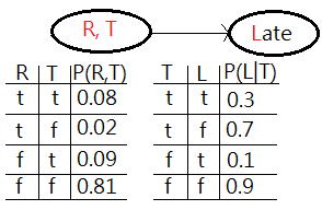
[2]The second is the operation of elimination, also called summing out or marginalization, to take the table $P(R,T)$, reduce it to $P(T)$, finally combine it with $P(L\vert T)$ to get $P(L)$.
➀by now, we sum out or marginalize $P(R,T)$ over the variable $R$ to get $P(T)$ that just operates on $T$. That is what we have in the network, by summing out over all values of $R$, respectively for which $T=t$ and $T=f$.
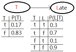 ➁next, we do a join over $T$ and $L$, by combining $P(T)$ and $P(L\vert T)$ to get a new factor of joint probability $P(T,L)$.
➂now, we are down to a network with a single node, $T,L$ with the joint probability table. By summing out $P(T,L)$ over $T$ with respect for $L=t$ and $L=f$, finally we reach the single node $L$ with $P(L=t)$ and $P(L=f)$.
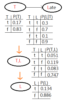
It is a continued process of joining together factors to form a maybe larger factor and then eliminating variables by summing out(marginalization).
Optimal Order For Variable Elimination Is NP-Hard
In this paragrapg, I’d like to illustrate the execution of different elimination order would probabilistically result in computational side effect. I’m going to use an example from Prof. Abbeel, steps through a few variable examples, but with my own viewpoint.
[Question]
The given BN is depicted below, what’s $P(U\vert +z)$?
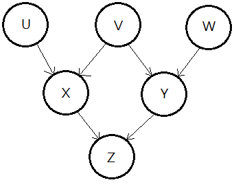 We are initialized with these factors, they are $P(U)$,$P(V)$,$P(W)$,$P(X\vert U,V)$,$P(Y\vert V,W)$,$P(Z\vert X,Y)$. Asking for $P(U\vert +z)$ is to eliminate the nodes of $X$,$Y$,$V$,$W$ in the network.
[Order: $X$,$Y$,$V$,$W$]
➀do the factor join over $X$ to eliminate $X$:
$f_{1}(+z,Y,U,V)$=$\sum_{x}P(+z\vert x,Y)\cdot P(x\vert U,V)$
There is a finding that the elimination of the node with multiple parents would generate a new factor with the number of extra added variables eqivalent to the number of its parents.
➁do the factor join over $Y$ to eliminate $Y$:
$f_{2}(+z,U,V,W)$=$\sum_{y}f_{1}(+z,y,U,V)\cdot P(y\vert V,W)$
➂do the factor join over $V$ to eliminate $V$:
$f_{3}(+z,U,W)$=$\sum_{v}f_{2}(+z,U,V,W)\cdot P(v)$
➃do the factor join over $W$ to eliminate $W$:
$f_{4}(+z,U)$=$\sum_{w}f_{3}(+z,U,W)\cdot P(w)$
➄we are left with $f_{4}(+z,U)$ and $P(U)$, then:
$P(U\vert +z)$=$\frac {P(U\cap +z)}{P(+z)}$, where $P(+z)$=$\sum_{u}f_{4}(+z,u)$ and $P(U\cap +z)$=$\sum_{u}f_{4}(+z,u)\cdot P(u)$. Be noted that this description won’t be repeated in below sections.
➅we can examine each new generated facor, inspect its scale, the width. Below exhibits each distinct generated factor’s number of variables.
 The maximum number in the new generated factor is 3, is such order the most optimal? Let’s continue to walk it through.
[Order: $V$,$W$,$X$,$Y$]
➀do the factor join over $V$ to eliminate $V$:
$f_{1}(X,U,Y,W)$=$\sum_{v}P(X\vert U,V)\cdot P(Y\vert V,W)\cdot P(V)$
There is another finding that the elimination of a node having more multiple children, then these children and their parents(if any), must be taken into computation cost.
➁do the factor join over $W$ to eliminate $W$:
$f_{2}(X,U,Y)$=$\sum_{w}f_{1}(X,U,Y,w)\cdot p(w)$
➂do the factor join over $X$ to eliminate $X$:
$f_{3}(+z,U,Y)$=$\sum_{x}f_{2}(X,U,Y)\cdot P(+z\vert x,Y)$
➃do the factor join over $Y$ to eliminate $Y$:
$f_{4}(+z,U)$=$\sum_{y}f_{3}(+z,U,y)$
➄you can follow [Order: $X$,$Y$,$V$,$W$]’s approach to renomalize for the answer.
➅we then examine each new generated facor, inspect its scale, the width. Below exhibits each distinct generated factor’s number of variables.
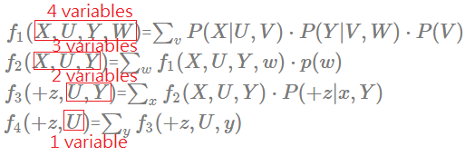 The maximum number in the new generated factor is 4, this elimination order is worse than $X$,$Y$,$V$,$W$ in computation efficiency. Let’s continue to walk it through to see if we can find another better one.
[Order: $W$,$V$,$Y$,$X$]
➀do the factor join over $W$ to eliminate $W$:
$f_{1}(Y,V)$=$\sum_{w}P(Y\vert V,w)\cdot P(w)$
➁do the factor join over $V$ to eliminate $V$:
$f_{2}(Y,X,U)$=$\sum_{v}f_{1}(Y,v)\cdot P(X\vert U,v)\cdot P(v)$
This is the same finding that the elimination of a node having more multiple children, then these children and their parents(if any), must be taken into computation cost.
➂do the factor join over $Y$ to eliminate $Y$:
$f_{3}(+z,X,U)$=$\sum_{y}f_{2}(y,X,U)\cdot P(+z\vert X,y)$
➃do the factor join over $X$ to eliminate $X$:
$f_{4}(+z,U)$=$\sum_{x}f_{3}(+z,X,U)$
➄you can follow [Order: $X$,$Y$,$V$,$W$]’s approach to renomalize for the answer.
➅we then examine each new generated facor, inspect its scale, the width. Below exhibits each distinct generated factor’s number of variables.
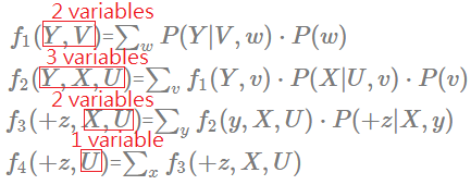 The maximum number in the new generated factor is 3, this elimination order is much betten than $V$,$W$,$X$,$Y$ in computation efficiency, and little better than $X$,$Y$,$V$,$W$. Let’s continue to walk it through to see if we can find another better one.
[Order: $W$,$Y$,$V$,$X$]
➀do the factor join over $W$ to eliminate $W$:
$f_{1}(Y,V)$=$\sum_{w}P(Y\vert V,w)\cdot P(w)$
➁do the factor join over $Y$ to eliminate $Y$:
$f_{2}(+z,X,V)$=$\sum_{y}f_{1}(y,V)\cdot P(+z\vert X,y)$
➂do the factor join over $V$ to eliminate $V$:
$f_{3}(+z,X,U)$=$\sum_{v}f_{2}(+z,X,v)\cdot P(X\vert U,v)\cdot P(v)$
➃do the factor join over $X$ to eliminate $X$:
$f_{4}(+z,U)$=$\sum_{x}f_{3}(+z,X,U)$
➄you can follow [Order: $X$,$Y$,$V$,$W$]’s approach to renomalize for the answer.
➅we then examine each new generated facor, inspect its scale, the width. Below exhibits each distinct generated factor’s number of variables.
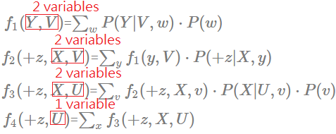 The maximum number in the new generated factor is 2, this elimination order is much betten than all previous orders. Let’s continue one more to see if we can find another better one.
[Order: $W$,$Y$,$X$,$V$]
➀do the factor join over $W$ to eliminate $W$:
$f_{1}(Y,V)$=$\sum_{w}P(Y\vert V,w)\cdot P(w)$
➁do the factor join over $Y$ to eliminate $Y$:
$f_{2}(+z,X,V)$=$\sum_{y}f_{1}(y,V)\cdot P(+z\vert X,y)$
➂do the factor join over $X$ to eliminate $X$:
$f_{3}(+z,U,V)$=$\sum_{x}f_{2}(+z,X,V)\cdot P(x\vert U,V)$
➃do the factor join over $V$ to eliminate $V$:
$f_{4}(+z,U)$=$\sum_{v}f_{3}(+z,U,V)\cdot P(v)$
➄you can follow [Order: $X$,$Y$,$V$,$W$]’s approach to renomalize for the answer.
➅we then examine each new generated facor, inspect its scale, the width. Below exhibits each distinct generated factor’s number of variables.
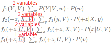 The maximum number in the new generated factor is 2, this elimination order is the same good as $W$,$Y$,$V$,$X$, much betten than all other orders. There exists total $4\cdot 3\cdot 2\cdot 1$ combinations.
So far, we reduce the scale(width) to 2 variables in the new generated factor should be confident to stop, since there should exist no factor ocntaining only 1 variable in this case!!
[Conclusion]
➀if we make the good choice of the order in which we apply these operations, then variable elimination can be much more efficient than just doing the whole enumeration!!
➁it’s an NP-hard issue to find an optimal order for variable elimination.
Variable Elimination Order Heuristics
The following heuristics are not the final solution to the most optimal order of variable elimination:
➀choose the variable with the fewest dependent variables.
➁choose the variable to minimize the product of cardinalities of its dependent or related variables.
➂choose the vertices to minimize the size of factors to be added in the graph.
Resort to related papers, textbooks, online references, I’d like to follow up Variable elimination, CS228, Stefano Ermon, instead of the complicated algorithm description and implementation here, since they are not jargon-free, you are welcome to my future article.
Addendum
➀Prof. Abbeel, steps through a few variable examples
➁Variable elimination, Peter Norvig
➂Bayesian Networks, Ben-Gal Irad, in Ruggeri F., Faltin F. & Kenett R., Encyclopedia of Statistics in Quality & Reliability, Wiley & Sons (2007).
➃Variable elimination, CS228, Stefano Ermon
In the incoming future, I might have my own version of algorithm.
➁eliminate variable $X$, we get the clique $(X,R)$:
➂eliminate variable $A$, we get the clique $(A,T)$:
➃eliminate variable $S$, we get the clique $(L,S,B)$, where the green line is the new pairwise connection after $S$ has been removed:
➄eliminate variable $D$, we get the clique $(R,D,B)$:
➅eliminate variable $B$, we get the clique $(L,R,B)$:
➆eliminate variable $L$, we get the final clique $(T,L,R)$:
Finally, connect the cliques thus obtained in accordance to the moralized MN.
➄eliminate variable $B$, we get the clique $(R,L,D,B)$, where the green line is the new pairwise connection after $B$ has been removed:
➅eliminate variable $D$, we get the clique $(R,L,D)$:
➆eliminate variable $L$, we get the final clique $(T,L,R)$:
Finally, connect the cliques thus obtained in accordance to the moralized MN(This might not be a perfect clique tree).
The functions associated with original clique tree are listed below:
➄eliminate variable $R$, we get the clique $(R,L,D,B)$.
➅eliminate variable $B$, we get the clique $(B,S,D)$.
➆eliminate variable $D$, we get the clique $(L,S,D)$.
Finally, connect the cliques thus obtained in accordance to the moralized MN(This might not be a perfect clique tree).
The functions associated with original clique tree could be found in prior section.
The ideal minimal clique tree would the illustration:
Current introduced buildCliqueTree() algorithm might not guarantee to have the minimal result, in the incoming future, I might develop a new algorithm for this. (to be conti…)
Below is the pre-requisite to next prove step:


 This is an invalid clique tree, variable B should exist in all the cliques in the path in between cliques of $(B,S)$ and $(R,D,B)$.
 This is a valid clique tree, since it meets the criteria that a variable could be found on all cliques in the path between 2 cliques containing it.
 ➀the union of the cliques is the set of the variables in the Bayesian network.
 Trivially, the multiplication of all functions on the clique tree is equivalent to the full joint probability distribution in the Bayesian network.
 If we take $\chi$ to be all unobserved variables, $P(\chi,E)$ is just the multiplication of all functions on the clique tess, which will laterly be proved.
 This exhibition reveals the portion mostly closed to the target pivot $C_{Q}$, the messages are coming from $C_{i}$, where $i$=$1$ to $k$, such message passing are triggered by the observed evidence on leaf nodes, maybe far away from these $C_{i}$s.
 The term $(C\cap C’)-E$ is better understood by this illustration. Since $C$ and $C'$ are independent, the intersection of the 2 nodes is null. It’s the evidence existing in the space in between $C$ and $C'$, after we minus $E$, what we want is the pure message from $C$ to $C'$.
 ➀do the join over $A=y$ in clique $(A,T)$:
 Using the same example of clique tree, the message is distributed from the pivot $(R,L,B)$ to all other cliques in reversed direction.
 ➀take $\chi$ to be the set of unobserved variables in all un-activated cliques, before $C$ send message to $C’$.
 ➄under ➃, we have $\chi$=$Z\cup\chi'$, the full illustration is exhibited below:
 ➅suppose property 2 is true that


 The point is that the total forward propoagated evidence from $X$ to $Y_{2}$ is the joint probability function in combinatory format of these 2 factors.

 The Markov network encodes the CPD in the Bayesian network as a factor of all related variables, like $P(E\vert B,C)$ is expressed in a factor form, $f(B,C,E)$, related variables in each distinct CDP are now be connected by an edge.
 , where $\phi_{1}$=$P(X_{1})$,$\phi_{2}$=$P(X_{2}\vert X_{1})$,$\phi_{3}$=$P(X_{3}\vert X_{1})$,$\phi_{4}$=$P(X_{4}\vert X_{2},X_{3})$,$\phi_{5}$=$P(X_{5}\vert X_{4})$.
 The goal of the most optimal variable elimination sequence is to introduce no extra fill-ins.
 Given this network, we’d like to prove $A\perp C\vert B$ given $P(A,B,C)$=$\frac {1}{Z}\cdot\phi_{A,B}(A,B)\cdot\phi_{B,C}(B,C)$:
 We can conclude that any BN conditioned on evidence can be regarded as a Markov network.
 To speed up the path to $P(U\vert +z)$, I use the optimal order of elimination: $W$,$Y$,$X$,$V$
 ➁eliminate the node $Y$.
 ➂eliminate the node $X$.
 ➃eliminate the node $V$.
 ➄therefore, we have:

 ➁next, we do a join over $T$ and $L$, by combining $P(T)$ and $P(L\vert T)$ to get a new factor of joint probability $P(T,L)$.
 We are initialized with these factors, they are $P(U)$,$P(V)$,$P(W)$,$P(X\vert U,V)$,$P(Y\vert V,W)$,$P(Z\vert X,Y)$. Asking for $P(U\vert +z)$ is to eliminate the nodes of $X$,$Y$,$V$,$W$ in the network.
 The maximum number in the new generated factor is 3, is such order the most optimal? Let’s continue to walk it through.
 The maximum number in the new generated factor is 4, this elimination order is worse than $X$,$Y$,$V$,$W$ in computation efficiency. Let’s continue to walk it through to see if we can find another better one.
 The maximum number in the new generated factor is 3, this elimination order is much betten than $V$,$W$,$X$,$Y$ in computation efficiency, and little better than $X$,$Y$,$V$,$W$. Let’s continue to walk it through to see if we can find another better one.
 The maximum number in the new generated factor is 2, this elimination order is much betten than all previous orders. Let’s continue one more to see if we can find another better one.
 The maximum number in the new generated factor is 2, this elimination order is the same good as $W$,$Y$,$V$,$X$, much betten than all other orders. There exists total $4\cdot 3\cdot 2\cdot 1$ combinations.