The Bayesian Network Profound Meaning

11 Jul 2018

Prologue To The Bayesian Network Profound Meaning

Bayesian networks(BNs), also known as belief networks(or Bayes nets for short), belong to the family of probabilistic graphical models(GMs), which are used to represent knowledge about an uncertain domain. BNs combine principles from graph theory, probability theory, computer science, and statistics.

Explaining Away

[1] Recap: d-separation

Accordingly, when one set of random variables, $\Theta_{1}$, is conditionally independent of another, $\Theta_{2}$, given a third, $\Theta_{3}$, then we say that the random variables in $\Theta_{1}$ are d-separated from $\Theta_{2}$ by $\Theta_{3}$. For the simplicity, you can treat each set containing only one random variable.

[2] Illustration of explaining away

Given that you got a headache, there exists more than a dozen of possible causes, the causal relationship is depicted below.
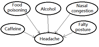➀suppose the inferred correct root cause to your headache is the nasal congestion.
➁the possibility of the rest nodes to be the root cause is greatly reduced, said they has been explained away.
➂given the evidence of a headache, some knowledge of food poisoning, caffeine, alcohol, faulty posture would be inferred from the state of nasal congestion and the observation of a headache.
➃they are no longer d-separated, but d-connected. Or they are conditionally dependent given a headache.

[3] Conclusion

D-connection in converging type networks requires some knowledge of the connection variable(the headache node in this example), at least one of the descendants, the observed evidence must have the positive or the negative information.

The Markov Blanket And Markov Equivalence

[1] Markov blanket

The Markov blanket claims a node is conditionally independent(d-separated) from all of the other nodes(entire graph), given its parents, childs, child's parents.
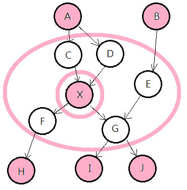➀in above graph, given nodes $C$, $D$, $E$, $F$, $G$, node $X$ is d-separated from all othere nodes, $A$, $B$, $H$, $I$, $J$.
➁the parents, the children, other parents of a node's children are called the Markov blanket of a node.
➂therefore Markov blanket contains all the variables that shields the target node from the rest of the network. This means that the Markov blanket of a target node is the only knowledge needed to predict the behavior of that target node.

Suppose we know the value of each node in the Markov blanket, if we’d like to predict the probability distribution of $X$, then there is no more information regarding to the value taken by the node $X$.

[2] Markov equivalence

Two DAGs are to be said Markov equivalent, if they have the same d-separations.

Prove The Markov Blanket

A node is conditionally independent of all other nodes given its Markov blanket, i.e. its parents, its children, and parents of common children(spouses).

proof::mjtsai1974

By using the same DAG of Markov blanket:
➀given target node’s parent, the target node is conditionally independent from the parent’s ascendant. $X$ is d-separated from $A$, given $C$ or $D$.
➁knowing $A$ could predict $C$, then from $C$ to predict $X$; knowing $X$ could infer $C$, then from $C$ to infer $A$. But, knowing $X$ helps nothing in inferring $A$, if we already know $C$; knowing $A$ makes no prediction about $X$, if we already know $C$.
➂given target node’s children, the target node is conditionally independent from the children’s descendants. $X$ is d-separated from $H$, given $F$, and is d-separated from $I$, $J$, given $G$. Similar in ➀.
➃given target node’s children, the children’s parent, the target node would be explained away, the same for that children’s parent, depends on the information on that children.
➄continue on, given $E$, $G$ is d-separated from $B$, then $X$ is also d-separated from $B$.

Therefore, the Markov blanket contains everything we need to predict and infer the target node.

Bayes Theorem With Background Context

[1] Incorporating the background context

Below is an intuitive Bayesian network:
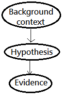We can deduce the posterior by incorporating the background context in the Bayes theorem expression:
$\;\;P(H\vert E,C)$=$\frac {P(E\vert H,C)\cdot P(H\vert C)}{P(E\vert C)}$

➀$C$, the background context.
➁$P(H\vert C)$, the hypothesis or prior term, based on the background context.
➂$P(E\vert H,C)$, the likelihood term, for the evidence, given the hypothesis and the background context.
➃$P(E\vert C)$, the total probability of evidence given the background context, and is independent of the hypothesis. It is the normalizing or scaling factor.
➄$P(H\vert E,C)$, the posterior term, the belief in hypothesis given evidence and the background context.

[2] Update probabilities of Bayesian network

In my prior post The Bayesian Inference Exploitation, I have exploited the process to update the prior(hypothesis) from the posterior.

New information about one or more nodes in the network updates the probability distributions over the possible values of each node. There are two ways in which information can propagate in a Bayesian network:
➀predictive propagation, it is straightforward, just by following the direction by the arrows. Once new information changes the probability of a node, the node will pass the information to its children, which in turn pass to its children, and so on.
➁retrospective propagation, it is an inverse of predictive propagation. Under retrospective propagation, when a node is updated, it will pass the information to its child node. But, if it is updated from the childe node, the information is passed to its parent node, and in turn pass to its parent node, and so on.

You can think of the update of information from one node to another is simultaneous(maybe atomic), if one node has multiple children, or parents.

Factorization In Bayesian Network

[1] Definition of DAG

According to the Introduction into Bayesian networks, p.6, Mgr. Libor Vaněk, we can define DAG as $G$=$(V,E)$, $V$ for the set of indices to random variables, $E$ for the edges, and $X$=$\{X_{v}: v\in V\}$ to be the set of random variables indexed by $v$.

[2] Factorization definition

$X$ is a Bayesian network with respect to $G$, if the model’s full joint probability density function could be expressed as a product of a series of the random variables’ PDFs(probability density functions), with each PDF having its probability conditionally depending on its parents:
$\;\;P(X)$=$\prod_{v\in V}P(X_{v}\vert pa(X_{v}))$, where $pa(X_{v})$ is the set of parents of $X_{v}$.

[3] Compare chain rule with conditional independence

Suppose $X$ has $n$ nodes in its network:
➀$P(X_{1}=x_{1},…,X_{n}=x_{n})$…by chain rule
=$\prod_{v=1}^{n}P(X_{v}=x_{v}\vert X_{v+1}=x_{v+1},…,X_{n}=x_{n})$
=$P(X_{1}=x_{1}\vert X_{2}=x_{2},…,X_{n}=x_{n})$
$\;\;\cdot P(X_{2}=x_{2}\vert X_{3}=x_{3},…,X_{n}=x_{n})$
$\;\;…$
$\;\;\cdot P(X_{n-1}=x_{n-1}\vert X_{n}=x_{n})$
➁$P(X_{1}=x_{1},…,X_{n}=x_{n})$…by factorization
=$\prod_{v=1}^{n}P(X_{v}\vert (X_{i1},X_{i2},X_{i3},…))$
; where $pa(X_{v})$=$\{X_{i1},X_{i2},X_{i3},…\}$

These 2 expressions differ in that the factorization of conditional independence for any descendant takes only its parents as the conditioning events, as I have shown it in the section “The Joint Probability Distribution Of Bayesian Network” in Introduction To The Bayesian Network.

Example: The Possible Causes To Computer Failure

This is an example from Bayesian networks, Michal Horný, Technical Report No. 5, April 18, 2014, which in turn simplified from Cowel et al, (1999). This example is illustrated here provided that I have a full implementation and explaination with the consistent result.

[Scene 1: the prior probability distribution, before evidence]

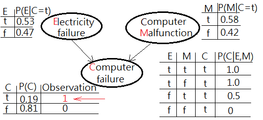
We are given a question of infering the possible root cause of computer failure(M), suppose the experiment comes with two possible suspects, electricity failure(E), computer malfunction(C):
➀the given prior, $P(E)$, $P(M)$ and the likelihoods of $P(C=t\vert E,M)$ are exhibited with the estimated probability for computer failure, $P(C)$ in below graph.
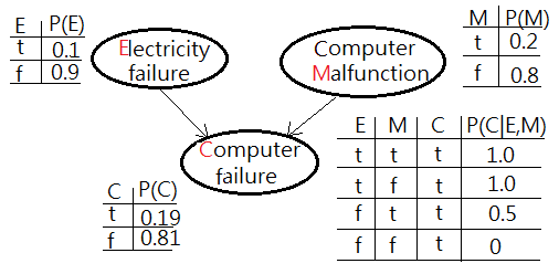➁$P(C=t)$
=$\sum_{E,M}P(C\vert E,M)\cdot P(E,M)$
=$\sum_{E,M}P(C\vert E,M)\cdot P(E)\cdot P(M)$
=$1\cdot 0.1\cdot 0.2$+$1\cdot 0.1\cdot 0.8$+$0\cdot 0.9\cdot 0.8$+$0.5\cdot 0.9\cdot 0.2$
=$0.02$+$0.08$+$0$+$0.09$
=$0.19$…the estimated probability of computer failure

[Scene 2: the posterior probability distribution, after evidence]

Assume we have been updated by the observation of physical computer failure, by the retrospective propagation, we could infer the possible root cause from the evidence.
➀$P(E=t\vert C=t)$
=$\sum_{M}P(E=t,M\vert C=t)$
=$\frac {\sum_{M}P(C=t\vert E=t,M)\cdot P(E=t)\cdot P(M)}{P(C=t)}$
=$\frac {1\cdot 0.1\cdot 0.2+1\cdot 0.1\cdot 0.8}{0.19}$
=$0.526315789$
$\approx 0.53$
➁$P(M=t\vert C=t)$
=$\sum_{E}P(M=t,E\vert C=t)$
=$\frac {\sum_{E}P(C=t\vert E,M=t)\cdot P(E)\cdot P(M=t)}{P(C=t)}$
=$\frac {1\cdot 0.1\cdot 0.2+0.5\cdot 0.9\cdot 0.2}{0.19}$
=$0.578947368$
$\approx 0.58$

The posterior of $P(M=t\vert C=t)$ is greater than $P(E=t\vert C=t)$ has been inferred by the observed evidence and depicted in below graph.

Example: The Possible Causes To Computer Failure And Light Failure

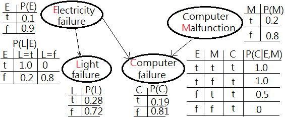
Extended from above example with one extra node of light failure(L) added in the network, conditionally dependent on electricity failure.

[Scene 1: the prior probability distribution, before evidence]

➀the given prior, $P(E)$, $P(M)$ and the likelihoods of $P(C=t\vert E,M)$, $P(L=t\vert E)$ are exhibited with the estimated probability for computer failure, $P(C)$, light failure, $P(L)$ in below graph. ➁$P(L=t)$
=$\sum_{E}P(L=t\vert)\cdot P(E)$
=$0.1\cdot 1.0+0.9\cdot 0.2$
=$0.28$…the estimated probability of light failure

[Scene 2: the posterior probability distribution, after evidence]

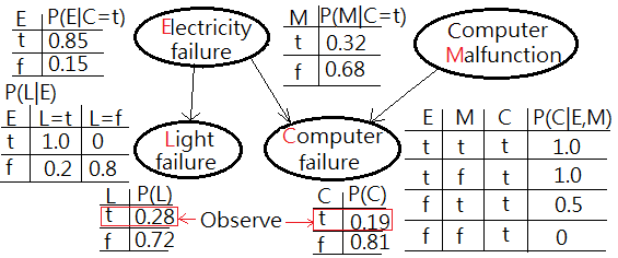
Assume we have been updated by the observation of physical computer failure and light failure, by the retrospective propagation, we could infer the possible root cause from the evidence.

Cautions must be made that the probability distribution and its expression has been changed as a result that the network has been new added a node. This is to ask for $P(E=t\vert C=t,L=t)$ and $P(M=t\vert C=t,L=t)$. I am going to take the advantage of factorization in the full joint joint PDF of this model:

➀$P(E=t\vert C=t,L=t)$=$\frac {E=t,C=t,L=t}{P(C=t,L=t)}$
,and $P(M=t\vert C=t,L=t)$=$\frac {M=t,C=t,L=t}{P(C=t,L=t)}$, for the commonality, we should deduce out the full joint PDF.
➁$P(E,M,C,L)$
=$P(L\vert E)\cdot P(C\vert E,M)\cdot P(E)\cdot P(M)$
➂$P(E=t,C=t,L=t)$
=$\sum_{M}P(E=t,M,C=t,L=t)$
=$P(L=t\vert E=t)\cdot P(C=t\vert E=t,M)\cdot P(E=t)\cdot P(M)$
=$1\cdot1\cdot 0.1\cdot 0.2+1\cdot 1\cdot 0.1\cdot 0.8$
=$0.1$
➃$P(C=t,L=t)$
=$\sum_{E}\sum_{M}P(E,M,C=t,L=t)$
=$\sum_{E}\sum_{M}P(L=t\vert E)\cdot P(C=t\vert E,M)\cdot P(E)\cdot P(M)$
=$1\cdot 1\cdot 0.1\cdot 0.2$
$\;\;$+$1\cdot 1\cdot 0.1\cdot 0.8$
$\;\;$+$0.2\cdot 0.5\cdot 0.9\cdot 0.2$
$\;\;$+$0.2\cdot 0\dot 0.9\cdot 0.8$
=$0.118$
➄$P(E=t\vert C=t,L=t)$
=$\frac {E=t,C=t,L=t}{P(C=t,L=t)}$
=$\frac {0.1}{0.118}$
=$0.847457627$
$\approx 0.85$
➅$P(M=t,C=t,L=t)$
=$\sum_{E}P(M=t,M,C=t,L=t)$
=$\sum_{E}P(L=t\vert E)\cdot P(C=t\vert E,M=t)\cdot P(E)\cdot P(M=t)$
=$1\cdot 1\cdot 0.1\cdot 0.2+0.2\cdot 0.5\cdot 0.9\cdot 0.2$
=$0.038$
➆$P(M=t\vert C=t,L=t)$
=$\frac {M=t,C=t,L=t}{P(C=t,L=t)}$
=$\frac {0.038}{0.118}$
=$0.322033898$

The posterior of $P(E=t\vert C=t,L=t)$ is greater than $P(M=t\vert C=t,L=t)$ has been inferred by the observed evidence and depicted in below graph.

Addendum

➀Bayesian networks, Michal Horný, Technical Report No. 5, April 18, 2014
➁Bayesian Networks, Ben-Gal Irad, in Ruggeri F., Faltin F. & Kenett R., Encyclopedia of Statistics in Quality & Reliability, Wiley & Sons (2007).
➂Introduction to discrete probability theory and Bayesian networks, Dr. Michael Ashcroft, September 15, 2011
➃Markov blanket
➄What are Bayesian belief networks?(part 1)
➅Introduction into Bayesian networks, Mgr. Libor Vaněk
➆Cowel R. G., Dawid A. P., Lauritzen S. L., Spiegelhalter D. J. (1999): Probabilistic Networks and Expert Systems. Springer-Verlag New York. ISBN 0-387-98767-3.

Introduction To The Bayesian Network

08 Jul 2018

Prologue To Introduction To The Bayesian Network

A Bayesian network is a model of a system, consisting of a number of random varaibles. It provides much more information than simple classifier(like neural networks, support vector machines), when used, the Bayesian network comes out with the probability distribution of the values of the random variable to be predicted.

What is a Bayesian Network?

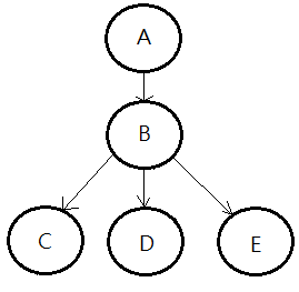
We begin by a simple graph illustration:
➀we can treat the it as a structured, graphical representation of probabilistic relationships between several random variables.
➁it explicitly encodes the conditional independences by the missing arcs.
➂it can efficiently represent the joint PDF(probability distribution function) of the whole network or the combinatorial random variables in the model.
➃it is a generative model, which allows arbitrary queries to be answered.

The Conditional Independence Relationship

In my previous article Introduction To The Conditional Probability, I have guided you through the conditional dependence. This article would then step into the field of conditional independence.

[1] Conditional independence axioms

A tutorial on Bayesian belief networks, Mark L Krieg, p.3 briefly describes the axiomatic basics for the conditional independence, which is in turn from the paper by Pearl, 1988.

Let $X$,$Y$,$Z$ denote any 3 distinct subsets of variables in the universe, called $U$. We define $I(X,Y,Z)_p$ to represent the conditional independence of $X$ from $Y$, given $Z$ in the probabilistic model $p$.
$\;\;I(X,Y,Z)_p$, iff $P(x\vert z,y)$=$P(x\vert z)$ and $P(y)>0$.

The following relationships holds:
➀$I(X,Z,Y)_p$
$\Leftrightarrow P(x,y\vert z)$=$P(x\vert z)\cdot P(y\vert z)$
➁$I(X,Z,Y)_p$
$\Leftrightarrow P(x,y,z)$=$P(x\vert z)\cdot P(y,z)$
➂$I(X,Z,Y)_p$
$\Leftrightarrow\;\exists f,g: P(x,y,z)$=$f(x,z)\cdot g(y,z)$, where $f,g$ are arbitrary functions of conditional probability or joint probability.

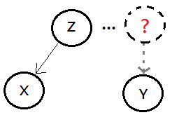
Above 3 equilibrium are based on the model that $X$ is the descendent of $Z$, where $Y$ is some unrelated node to both $X$,$Z$.

[2] 3 dependencies

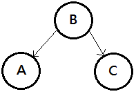
They could be treated as 3 types of connections in the Bayesian network, they are:
➀serial connection, knowing $B$ makes $A$ and $C$ independent, this is the intermediate cause.
➁diverging connection, knowing $B$ makes $A$ and $C$ independent, this is the common cause.
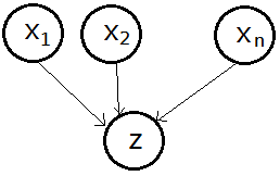
➂converging connection, this is the common effect, not knowing $Y$ makes $X_{1}$,$X_{2}$,...,$X_{n}$ independent.

The Bayesian Network=$(G,\Theta)$

In this article, we define $(G,\Theta)$ of the Bayesian networks to be the graphic representation of models capturing the relationships in between model’s variables, where:
➀$G$ is the DAG(directed acyclic graphic) containing nodes connected by arcs with arrows, the nodes are the random variables, the direction of arcs begins from parent node(s) to its descendent nodes, the child node depends on its parent node.
➁$\Theta$ is the set of parameters in all conditional probability distributions.

Where the DAG is the graphic containing no node of self-recycling path.

The Joint Probability Distribution Of Bayesian Network

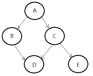
Continue to use above DAG, I’d like to compute the joint probability of all random variables in this Bayesian network, I’m going to illustrate each step of proof:

proof::mjtsai1974

[1]By chain rule, we have:
$P(A,B,C,D,E)$
=$P(E\vert D,C,B,A)$
$\;\;\cdot P(D\vert C,B,A)$
$\;\;\cdot P(C\vert B,A)$
$\;\;\cdot P(B\vert A)$
$\;\;\cdot P(A)$

[2]By the conditional independence in this model, we can further simplify these terms:
➀$P(E\vert D,C,B,A)$=$P(E\vert C)$
➁$P(D\vert C,B,A)$=$P(D\vert C,B)$
➂$P(C\vert B,A)$=$P(C\vert A)$
➃therefore, the full joint probability is thus expressed:
$P(A,B,C,D,E)$
=$P(E\vert C)$
$\;\;\cdot P(D\vert C,B)$
$\;\;\cdot P(C\vert A)$
$\;\;\cdot P(B\vert A)$
$\;\;\cdot P(A)$

The Number Of Parameters In The Bayesian Network

In the Bayesian network, each node represents a random variable, each arc encodes the conditional dependency in between parent and child nodes.

Succeeding to the same DAG, I’d like to decode out the number of parameters encoded in the conditional dependencies in the model, to which the network is trying to approximate.
➀the parameters are not equivalent to the nodes of random variables.
➁the parameters are the compounded conditioning events, depicted in below graph.
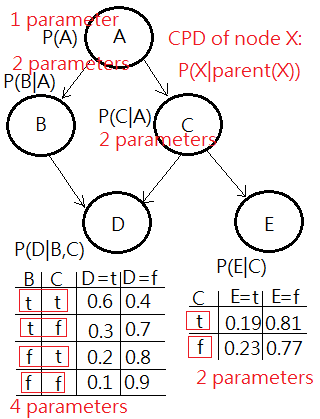➂totally, $1$+$2$+$2$+$4$+$2$, there are $11$ parameters in this probabilistic model of network, compared to the multinomial distruibution, in this case $2^{5}-1$=$31$ parameters.

Such a reduction provides benefits from inference, learning(parameter estimation) and compuutation perspective.

The Concept Of D-Separation

[1] d-separated

Nodes $X$ and $Y$ are d-separated, if on any (undirected)path in between $X$ and $Y$, there exists some random variable $Z$, such that:
➀$Z$ is in a series or diverging connection and $Z$ is known, or
➁$Z$ is in a converging connection, neither $Z$ nor any of its descendent(s) $W$ is known.
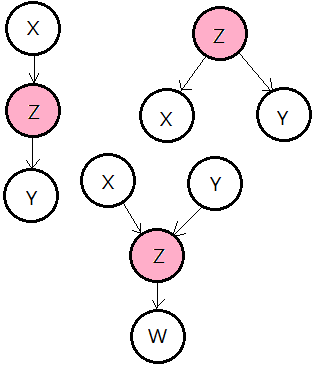There is one alternative condition, that $Z$ is not known, $X$, $Y$ and $W$ are all d-separated.

[2] d-connected

Nodes $X$ and $Y$ are d-connected, if they are not d-separated. The most trivial example is that $Y$ is the descendent of $X$.

[3] conditional independence

Nodes $X$ and $Y$ are d-separated by $Z$, then they are conditionally independent given $Z$.

Addendum

➀A tutorial on Bayesian belief networks, Mark L Krieg
➁A tutorial on learning and inference in the Bayesian networks, Irina Rish

The Bayesian Inference Exploitation

17 Jun 2018

Prologue To The Bayesian Inference Exploitation

Bayesian inference is resembling gradient descendent approach to guide the experiment to the target satisfication, they are not the same, but alike!

Prepare to Exploit The Bayesian Inference

[1] ReCap The bayesian inference

We can characterize how one’s beliefs ought to change when new information is gained.

Remember the illustration example in the The Bayesian Thinking, I have show you by contiguous update the given prior by the estimated posterior would we obtain the desired result by reinforcement.

[2] The question in mind

From #1, #2, #3 tests, by feeding the prior with the positive posterior estimation, then we get almost $100\%$ in $P(Cancer\vert Malignant)$. Below are the unknowns:
➀how, if we update the given prior several times with the positive posterior estimation, $P(Cancer\vert Malignant)$, laterly make contiguous negative posterior estimation, $P(Cancer\vert Benign)$?
➁will we have the chance to increase the negative posterior estimation, in its probability, $P(Cancer\vert Benign)$?
➂for the answer of yes and no, could we describe the exact trend of $P(Cancer\vert Benign)$?
➃or, is there some condition far beyond our naive beliefs that prior updated by some amount of positive posterior, we can concrete the negative posterior?

[3] The stress test

Below is my stress test flow:
➀the rule of updating prior by the estimated posterior remains the same, when we make estimation of $P(Cancer\vert Malignant)$ and $P(Cancer\vert Benigh)$, at the end of each test, we do the update job.
➁by executing $P(Cancer\vert Malignant)$ in $i$ times, next to execute $P(Cancer\vert Benign)$ over $100-i$, where $i$=$1$ to $100$.
➂below graph exhibits the result of $P(Cancer\vert Malignant)$x${i}$, $P(Cancer\vert Benign)$x$(100-i)$ for the first 12 tests:
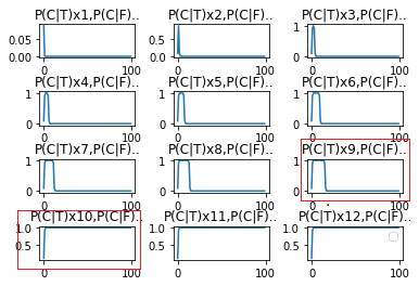The results are depicting from the left, top to the right, low in orders. For the simplicity, I denote $P(C\vert T)$ as $P(Cancer\vert Malignant)$, $P(Cancer\vert F)$ as $P(Cancer\vert Benign)$.
➃trivially, $P(C\vert T)$x$9$ to $P(C\vert T)$x$10$ is the major point, after positive posterior over $10$ times, the following negative posterior won't be decreased, and keeps the same result as the latest positive posterior!

Exploit The Bayesian Inference

Next we investigate what positive posterior over $10$ times has put inside the whole process, such that the following up $90$ negative posteriors would not downgrade the probabilistity of $P(Cancer\vert Benigh)$.

[1]By comparing the statistical log info of $P(C\vert T)$x$9$ and $P(C\vert T)$x$10$
The test is 0-index based in my log, so you see run 9 is actually the 10-th execution of the test:
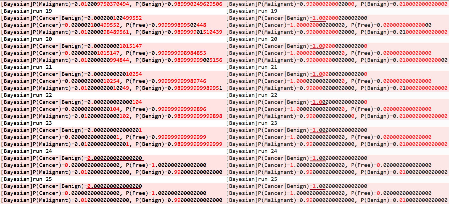
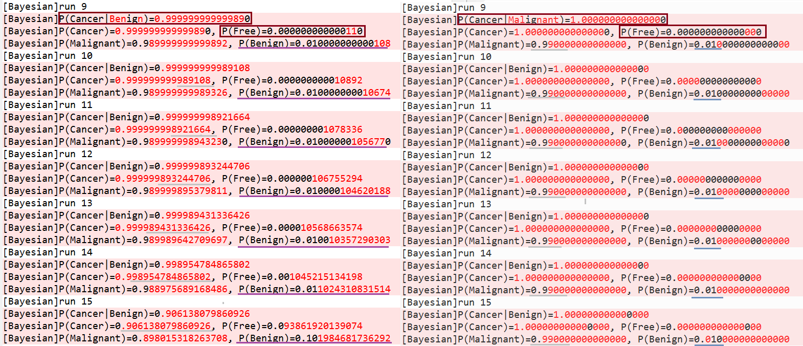➀the log comparison reveals that the run #9 in $P(C\vert T)$x$9$, the left side, says $P(Cancer\vert Benign)$ is almost $1$, but not yet!
➁the right side result, the run #9 in $P(C\vert T)$x$10$ says $P(Cancer\vert Malignant)$ is equivalent to $1$!
➂the left side $P(C\vert F)$x$9$ has its $P(Cancer)$ and the total probability of $P(Malignant)$ downgraded, since the negative posterior is thus estimated:
$P(Cancer\vert Benign)$=$\frac {P(Benign\vert Cancer)\cdot P(Cancer)}{P(Benign)}$
$P(Benign)$=$P(Benign\vert Cancer)\cdot P(Cancer)$
$\;\;\;\;$+$P(Benign\vert Free)\cdot P(Free)$

The $P(Free)$ and $P(Benign)$ are compounded slowly increasing, the root cause to gradually decrease $P(Cancer\vert Benign)$!!

➃the right side $P(C\vert T)$x$10$, from the run #9(10-th) test of $P(Cancer\vert Malignant)$, we have $P(Cancer)$=$1$, $P(Free)$=$0$ keep invariant change in the total probability of $P(Malignant)$ and $P(Benign)$.
➄continue to inspect the log comparison result, we can see that in the series of $P(C\vert T)$x$9$, $P(C\vert F)$x$91$, the negative posterior becomes smaller and finally to 0; nevertheless, the $P(C\vert T)$x$10$, $P(C\vert F)$x$90$, we have $P(Cancer\vert Benign)$=$1$ all the way to the test end.

[2]Deeper inside $P(C\vert T)$x$9$ and $P(C\vert T)$x$10$
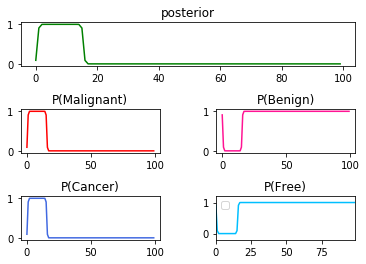
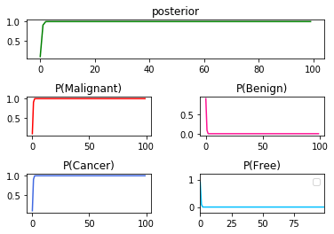
To make my findings concrete, the statistical summary of the 2 series are given in below graphs:
➀below graph illustrates the consistency of my finding is of no doubt in $P(C\vert T)$x$9$.
➁the same in $P(C\vert T)$x$10$.

[3]Other testing reports
At the end of this article, I depict all stress test I have done.
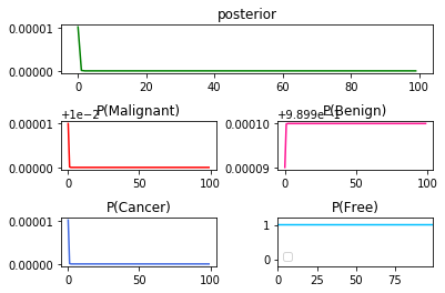
➀it is the result of $P(Cancer\vert Malignant)$x$100$:
➁it is the result of $P(Cancer\vert Benign)$x$100$:
➂below exhibits the result in the series $P(Cancer\vert Malignant)$x$50$, then $P(Cancer\vert Benign)$x$50$:
➃the result in the series $P(Cancer\vert Malignant)$,then $P(Cancer\vert Benign)$ as a whole the pattern for the behavior in the rest process:
You can tell that the patterned toggling exist for all terms of probability.

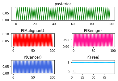
All above reports are generated by my Python simulator. The related logs are downloaded here, $P(Cancer\vert Malignant)$ over $9$ times and $P(Cancer\vert Malignant)$ over $10$ times.

The Bayesian Thinking

11 Jun 2018

Prologue To The Bayesian Thinking

Bayesian thinking is an approach to systematizing reasoning under uncertainty by means of the Bayes theorem.

The Intuition Behind The Bayes Theorem

[1] ReCap the Bayes theorem

The detailed explanation of 4 factors are in my prior post, The Bayes Theorem Significance.

[2] The intuition behind the theorem

The intuition behind encourages you to make further inference.
➀the hypothesis, mapped to the prior, which are all probabilities.
➁the likelihood function related to prior is expressed as the probability of the event occurrence of the observation given the event occurrence of hypothesis.
➂the total probability of the observation is the well regularized evidence.
➃the posterior is the probability of the hypothesis, given the observation.

[3] The Bayesian inference

➀at the first glance, we make an observation in the real world.
➁we’d like to identify it by making certain hypothesis of some classification.
➂the likelihood function estimates the possible probability of the observation given the hypothesis.
➃finally, the posterior is the probability of the hypothesis given the observation.
Such process is called the Bayesian inference, full compliant with the classification of an observed object, which the hypothesis is made all about.

By the way, observation, hypothesis, likelihood function are all based on the qualitative belief, the total probability of the observation and the posterior are the quantitative outcomes.

The Bayesian Inference Illustration

My illustration in this article was inspired from Introduction to Bayesian Thinking: from Bayes theorem to Bayes networks, Felipe Sanchez, it is using an example from The Anatomy Of Bayes Theorem, The Cthaeh. But, I have some different opinion.

[1] Begin by a question

➀suppose everyone could casually find some mass in your body, like skin. It might be a rare disease, according to the medical library, only 1 from 1000 people having a mass would be the cancer, given in below table.

	Probability
Cancer	0.001
Mass	0.999

This table reveals the already known prior, now turns into be the hypothesis of the probability of having a cancer.
➁suppose the accuracy of the medical detection is given in below table, where malignant stands for cancer of result, and benign stands for being detected as a normal mass.

	Cancer	Mass
Malignant (Cancer)	$P(Malignant\vert Cancer)$=0.99	$P(Malignant\vert Mass)$=0.01
Benign (Not a cancer)	$P(Benign\vert Cancer)=0.01$	$P(Benign\vert Mass)$=0.99

This table directly reflects the possible likelihood for all conditional combinations of 2 observations, malignant and benign.
➂unfortunately, you are detected as having a cancer, then, what's the probability that you are really having a cancer given that you are medically detected as a victim of cancer?
This given question is asking for $P(Cancer\vert Malignant)$, which is the posterior.

[2] Test of run #1

By the given hypothesis, likelihood, the Bayes theorem could be used for the posterior:
➀$P(Cancer\vert Malignant)$
=$\frac {P(Malignant\vert Cancer)\cdot P(Cancer)}{P(Malignant)}$
➁the total probability of malignant evidence:
$P(Malignant)$
=$P(Malignant\vert Cancer)\cdot P(Cancer)$+$P(Malignant\vert Mass)\cdot P(Mass)$
➂therefore, the posterior is
$P(Cancer\vert Malignant)$
=$\frac {0.99\cdot 0.001}{0.99\cdot 0.001+0.01\cdot 0.999}$=$0.090163$
; where $P(Mass\vert Malignant)$=$0.909837$, take it as $0.91$ after rounding.

[3] Test of run #2

Even if the accuracy of the medical detection is up to $0.99$, the probability for your mass is really a cancer given the malignant diagnostic result is only $0.09$. That’s why we decide to make the 2nd test.
➀first, we update the prior table with regard to the given run #1 result:

	Probability
Cancer	0.09
Mass	0.91

It is under the assumption that the run #1 is rather a plausible, not a vague result!!
➁recalculate with the Bayes theorem:
$P(Cancer\vert Malignant)$
=$\frac {0.99\cdot 0.09}{0.99\cdot 0.09+0.01\cdot 0.91}$
=$0.90733$
$\approx 0.91$
; where $P(Mass\vert Malignant)$=$0.09266\approx 0.09$, after rounding. Wow, it seems there is a great improvement in a malignant report and you do really have a cancer.

[4] Test of run #3

Let’s do it the 3rd run.
➀first, we update the prior table with regard to the given run #2 result:

	Probability
Cancer	0.91
Mass	0.09

It is under the assumption that the run #2 is rather a plausible, not a vague result!!
➁recalculate with the Bayes theorem:
$P(Cancer\vert Malignant)$
=$\frac {0.99\cdot 0.91}{0.99\cdot 0.91+0.01\cdot 0.09}$
=$0.999$
$\approx 1$
; where $P(Mass\vert Malignant)$=$0.0001$, after rounding.
It is now almost $100\%$ correct that the malignant report says that you have a cancer!!!

[5] Summary

This illustration begins with the given prior of having cancer, executes from run #1 to run #3, constantly updates the next prior probability with the current estimated posterior, finally get the expected result. It is called the Bayesian inference.

The Review::mjtsai1974

Above illustration of Bayesian inference might strike you on your head that by constantly updating the given prior(so that you can make finer hypothesis) would you gradually adjust the posterior(the experiment result) toward the direction you want.

[Question]

Below I comment out with 2 doubtable points:
➀why we update the prior, $P(Cancer)$ with $P(Cancel\vert Malignant)$ after each test?
➁is this the artificial bias leads to the contribution of $100\%$ identification of having a cancer given the malignant result?

[Answer]

➀I think it is indeed an artificial bias, since the term $P(Cancer\vert Malignant)$ is not equivalent to the very first given $P(Cancer)$ for all possible diseases one can have as a sample or population.
➁be remembered that it is the common practices in Bayesian inference.

Addendum

➀Introduction to Bayesian Thinking: from Bayes theorem to Bayes networks, Felipe Sanchez
➁The Bayesian trap, Veritasium channel
➂The Anatomy Of Bayes Theorem, The Cthaeh

Bayes From Theorem To Practice

06 Jun 2018

Prologue To Bayes From Theorem To Practice

The Bayes theorem is the quantitative critical thinking rather than the qualitative thinking of human nature. By using already known probability of feature to figure out unknown probability of interested feature in its maximum likelihood, the result would be more plausible.

You Are Given The Question

Given a dog, with 3 measurement results(lb) of weight, $13.9$,$17.5$,$14.1$ in the past 3 records of measurement. What's the exact weight of the dog at this moment? And the scale tells that it is weighted 14.2 lb in this concurrent measurement.

This article is illustrated from the example in How Bayesian inference works, Brandon Rohrer.

Can We Try The Unbiased Estimator?

[1]Since we are given a sample of $13.9$,$17.5$,$14.1$, how about the unbiased estimator?
➀by $\frac {X_{1}+X_{2}+X_{3}}{3}$=$\overline{X_{3}}$, this is to use sample average to approximate the mean. The current drawback might be that we have sample of only a few data.
➁next we look at sample variance:
$\frac {\sum_{i=1}^{n}(X_{i}-\overline{X_{n})^{2}}}{n-1}$=$S_{n}^{2}$,
where $S_{n}^{2}$ is the sample variance.
➂next we look at sample standard deviation:
$S_{n}$=$(\frac {\sum_{i=1}^{n}(X_{i}-\overline{X_{n})^{2}}}{n-1})^{\frac {1}{2}}$ is the sample standard deviation, $n$=$3$ in this example.
➃then, the the standard error term:
$se$=$(\frac {\sum_{i=1}^{n}(X_{i}-\overline{X_{n})^{2}}}{n})^{\frac {1}{2}}$, is the standard error in this sample.

[2]All above are major terms in modern probability and statistics, and the standard error term have another expression in linear regression:
➀suppose $Y$ is the real target, and $\widehat Y$ is the estimated value of target, in linear regression, the term $RSS$=$\sum_{i=1}^{n} (Y_{i}-\widehat Y_{i})^{2}$ is the residual sum of squares.
➁we denote $(\frac {RSS}{dof})^{\frac {1}{2}}$ as the the standard error in linear regression. In this example, $dof$ is unknown, since we have not yet build a linear regression model. By intuition, $dof$=$2$, because there is an average $\overline{X_{3}}$ taken into account.

[3]After simple calculation, we have:
➀$\overline{x_{3}}$=$15.167$, the little case of letter $x$ indicates the value.
➁$S_{n}^{2}$=$4.09333351$
➂$S_{n}$=$2.023$
➃$se$=$1.6519$

Before We Start

[1]We’d like to evaluate the possible accurate weight. By given, we have 3 already known weights in the sample. Suppose the weights are in normal distribution.
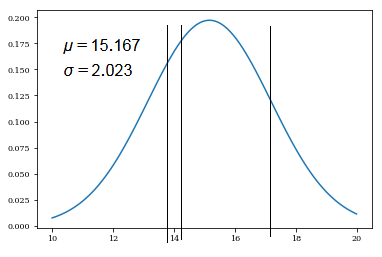
➀by $\overline{x_{3}}$=$15.167$, $S_{n}$=$2.023$, the shape of normal distribution is exhibited below:
➁by $\overline{x_{3}}$=$15.167$, $se$=$1.6519$, the shape of normal distribution is exhibited below:
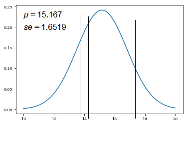The shape of normal distribution is more sharpen, if we use the population standard deviation(standard error) to be the standard deviation, which is smaller, this indicates some bias exists in between 2 sources of standard deviation, they are sample standard deviation and the population standard deviation(standard error).

[2]We have 3 already known weights in the sample, what are $P(13.9)$,$P(14.1)$ and $P(17.5)$?
➀should we treat $P(13.9)$=$P(14.1)$=$P(17.5)$=$\frac {1}{3}$? Since each measurement comes out with one value of weight, the occurrence of getting the weight.
➁or by using $\frac {1}{\sigma\cdot\sqrt {2\cdot \pi}}\cdot e^{-\frac {(x-\mu)^{2}}{2\cdot\sigma^{2}}}$ to calculate the respective probability?

There is no standard answer, yet!!!

Translate The Target Into The Correct Probabilistic Expression

It seems that the target of accurate weight is very clear, but, how to translate into the correct probabilistic expression is the major topic.
We denote $w$ to represent the weight, $m$ as each measurement. How to express the weight each time the dog is measured? It is determinant in the prior and the target posterior. Below lists 2 of my viewpoints:
[1]$P(w\vert m)$=$\frac {P(m\vert w)\cdot P(w)}{P(m)}$
➀this is to ask the maximum probability of the real weight from the given measurement, the target posterior is $P(w\vert m)$, and the $P(w)$ is the already known weight(lb), the prior.
➁suppose the measurement process is under certain quality control, and we no doubt the result.

[2]$P(m\vert w)$=$\frac {P(w\vert m)\cdot P(m)}{P(w)}$
➀this is to ask the maximum probability of the accuracy of the measurement result from the given weight(to be believed such quantitative weight is verified and correct), the target posterior is $P(m\vert w)$, and the $P(m)$ is the already known measurement result(lb), the prior.
➁the major purpose of this expression should work when we'd like to evaluate the accuracy of the measurement process or result, it’s the condition that we doubt the measurement result, we’d like to make further enhancement in the measurement equipment or the process.

[3]Therefore, we choose $P(w\vert m)$=$\frac {P(m\vert w)\cdot P(w)}{P(m)}$ as our Bayes expression, and $P(m\vert w)$ is the likelihood function for the probability of the measurement outcomes, $13.9$,$17.5$,$14.1$, given the true weight $w$.

A Dead Corner Leading To Nowhere

[1] We are still in a no-escape corner, why?

By choosing $P(w\vert m)$=$\frac {P(m\vert w)\cdot P(w)}{P(m)}$ as our Bayes expression only makes it a point in intuition layer.
➀we don’t know how to make $P(w)$,$P(m)$,$P(m\vert w)$ quantitative.
➁should we treat $P(m\vert w)$ to be in uniform or Gaussian distribution?

[2] Try to escape.

To be compliant with the Bayes expression of our choice, let’s back to the inference for the total probability $P(m)$ of the measurement.
➀suppose the dog’s weight would vary by time, thus we are given 3 different measurement results of weight.
$P(m)$=$P(m\vert w_{1})\cdot P(w_{1})$+$P(m\vert w_{2})\cdot P(w_{2})$+$P(m\vert w_{3})\cdot P(w_{3})$
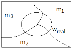
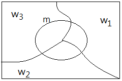➁we believe there exists indeed a true value of dog's weight, $w_{real}$. Base on the total probability of these 3 measurements, we’d like to estimate out the probability of such $w_{real}$ by $P(w_{real}\vert m)$.
➂to further regularize our Bayes expression, let it becomes:
$P(w_{real}\vert m)$=$\frac {P(m\vert w_{real})\cdot P(w)}{P(m)}$, where $P(m)$ and $P(w_{real})$ are just constants.
➃we can toss out the 2 terms $P(m)$ and $P(w_{real})$. The working model now becomes:
$P(w_{real}\vert m)$=$P(m\vert w_{real})$

It's the possible direction we can escape away from the space non-going anywhere, as a result of the chosen Bayes expression constructed by insufficient sample data.

The Maximum Likelihood For $P(w_{real}\vert m)$

[1] The working model filled with given data

$P(w_{real}\vert m)$=$P(m\vert w_{real})$ leads us to the maximum likely possible real weight.
➀fill in what we are given:
$P(w_{real}\vert m=\{13.9,14.1,17.5\})$
=$P(m=\{13.9,14.1,17.5\}\vert w_{real})$
➁next to interpret $P(m\vert w_{real})$ by the Gaussian normal distribution.

Because this is fully compliant with the assumption that the accuracy of measurement result of weight is of no concern, and the weight varies by time, thus come out with different results.

[2] The way to do the maximum likelihood estimation

➀it is to be proceeded with a given possible real weight, to generate the maximum value of $P(m=\{13.9,14.1,17.5\}\vert w_{real})$, and such $w_{real}$ will yield the largest probability of $P(w_{real}\vert m=\{13.9,14.1,17.5\})$.
➁$\underset{w_{real}}{maxarg}P(m=\{13.9,14.1,17.5\}\vert w_{real})$
=$\underset{w_{real}}{maxarg}P(m=\{13.9\}\vert w_{real})$
$\;\;\;\;\cdot P(m=\{14.1\}\vert w_{real})$
$\;\;\;\;\cdot P(m=\{17.5\}\vert w_{real})$
This is just the maximum likelihood estimation for $w_{real}$.
➂to have more probability and be centralized toward the $\overline{X_{3}}$, this article choose $\overline{x_{3}}$=$15.167$, $se$=$1.6519$ to build the Gaussian normal distribution.
Take $w_{real}\in\{\overline{X_{3}}\pm se\}$, ranges from $13.5151$ to $16.8189$.
➃it’s not inclusive of the given measurement result $17.5$, to make it more complete:
$w_{real}$=$\{13,…,18\}$
➄let the data or the experiment result speaks!!

In my Python simulator, the maximum likelihood estimation of $w_{real}$ is $15.126$, for whatever sample or population standard deviation we choose to make the normal distribution.
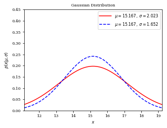The estimated $w_{real}$=$15.126$, which is very close to $\overline{x_{3}}$=$15.167$, is this the most appropriate value?

Make The Bayes Inference With The Given Prior

[1] The Bayes inference should begin with the given prior

Please recall that the scale tells the dog is weighted $14.2$ lb in this concurrent measurement, and this is the prior to make Bayes inference with.
➀assumed the given prior $P(w_{real})$=$14.2$ is true.
➁since $14.2$ is within the existing sample space, we can just take $\mu$=$14.2$ and the same sample or population standard deviation to build the mother normal distribution.

[2] Refine the working model

$P(w_{real}\vert m)$=$P(m\vert w_{real})\cdot P(w_{real})$
➀the Bayes inference should begin with the given prior, that’s why we put the term P(w_{real}) at the right side.
➁the term $P(m)$ is just a constant, could be safely tossed out.

[3] Design the new flow

We’ll still use the maximum likelihood estimation for the real weight, there will be some flow change:
➀take $\mu$=$14.2$ and the same sample or population standard deviation to build the mother normal distribution to simulate the real weight.
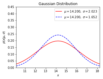The red solid line is the normal distribution of sample standard deviation, the dashed blue line is the version of population standard deviation.
➁iterate through each measured weight in the sample space.
➂take the current iterated measured weight as $\mu$ to build a new normal distribution, centrally distributed in accordance with it.
➃calculate the $P(w_{cur})$ with regards to the normal probability distributed in the normal distribution build in ➀.
➄calculate the standard deviation in this new build normal distribution.
$P_{\mu=14.2}(17.5)$=$\frac {1}{\sigma_{\mu=17.5}\cdot\sqrt{2\cdot\pi}}\cdot e^{-\frac {1}{2}\cdot\frac {(x-17.5)}{\sigma_{\mu=17.5}^{2}}}$
$\Rightarrow\sigma_{\mu=17.5}$=$\frac {1}{P_{\mu=14.2}(17.5)\cdot\sqrt{2\cdot\pi}}$
;where $x=17.5$ and $P_{\mu=14.2}(17.5)$=$\frac {1}{\sigma_{\mu=14.2}\cdot\sqrt{2\cdot\pi}}\cdot e^{-\frac {1}{2}\cdot\frac {(17.5-14.2)}{\sigma_{\mu=14.2}^{2}}}$
thus, we can know the bandwidth of normal distribution regarding to $\mu$=$17.5$.
After the calculation with sample standard deviation $2.023$, we have $\sigma_{\mu=13.9}$=$2.046$, $\sigma_{\mu=14.1}$=$2.026$, $\sigma_{\mu=17.5}$=$7.651$.
And calculate with population standard deviation $1.652$, we have $\sigma_{\mu=13.9}$=$1.679$, $\sigma_{\mu=14.1}$=$1.655$, $\sigma_{\mu=17.5}$=$12.149$.
➅by using the maximum likelihood estimation(see [4]) to find out the maximum $P(w_{real})$:
$P(w_{real}\vert m)$=$P(m\vert w_{real}\cdot w_{real})$
➆back to ➁ until all sample weights are iterated.

[4] Bayes maximum likelihood estimation

$P(w_{real}\vert m)$=$P(m\vert w_{real})\cdot P(w_{real})$ leads us to the maximum likely possible real weight.
➀when iterating $17.5$, $w_{real}$=$17.5$.
$P(w_{real}\vert m=\{13.9,14.1,17.5\})$
=$P(m=\{13.9,14.1,17.5\}\vert w_{real})\cdot P(w_{real})$
=$P_{N(\mu=17.5)}(m=\{13.9\}\vert 17.5)\cdot P_{N(\mu=14.2)}(17.5)$
$\;\;\;\;\cdot P_{N(\mu=17.5)}(m=\{14.1\}\vert 17.5)\cdot P_{N(\mu=14.2)}(17.5)$
$\;\;\;\;\cdot P_{N(\mu=17.5)}(m=\{17.5\}\vert 17.5)\cdot P_{N(\mu=14.2)}(17.5)$
➁let’s regularize it:
$\underset{w_{real}}{maxarg}P(m=\{13.9,14.1,17.5\}\vert w_{real})$
=$\underset{w_{real}}{maxarg}P(m=\{13.9\}\vert w_{real})\cdot P(w_{real})$
$\;\;\;\;\cdot P(m=\{14.1\}\vert w_{real})\cdot P(w_{real})$
$\;\;\;\;\cdot P(m=\{17.5\}\vert w_{real})\cdot P(w_{real})$
This is just the maximum likelihood estimation for $w_{real}$ in this Bayes inference.
➂below exhibits the new distribution with regards to all sampling weights and the mother sample standard deviation.
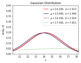Next it depects the new distribution with regards to all sampling weights and the mother population standard deviation.
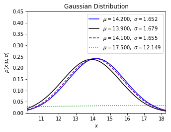Trivially, the new distribution centralized at $17.5$ has less, only a few probability to be the real weight.

In my Python simulator, the maximum likelihood estimation of $w_{real}$ is $14.1$, for whatever sample or population standard deviation we choose to make the mother normal distribution.

It seems that the final posterior is determinant by the given prior.

Addendum

➀How Bayesian inference works, Brandon Rohrer
➁Translated article of ➀
➂Bayes theorem and conditional probability