The Bayes Theorem Significance

28 May 2018

Prologue To The Bayes Theorem Significance

The most optimized effect of Bayes theorem is to use already known probability to figure out the maximum unknown probability in its likelihood, instead of manual counting in the sample space. The Bayes theorem is the weapon for quantitative critical thinking to overcome the drawback of qualitative thinking of human nature.

The Bayes Theorem Significance

$\;\;\;\;P(B_{i}\vert A)$=$\frac {P(A\vert B_{i})\cdot P(B_{i})}{P(A\vert B_{1})\cdot P(B_{1})+…+P(A\vert B_{n})\cdot P(B_{n})}$
[1] The general form of Bayes theorem embedes a total probability expression in its denominator part.
➀such total probability is the linear combination of the events in the sample space with the probability $P(A\vert B_{i})$, the occurrence of the target condition $A$, under the given partitioned sample space $B_{i}$ as it’s weighting.
➁usually, $A$ is the qualitative feature of interest.
➂$\Omega$=$\{B_{1},B_{2},…,B_{n}\}$, where $B_{i}$ is the partition os the sample space.
[2] The general form of Bayes theorem has joint probability expression in its nominator part.
➀the joint probability is expressed in terms of $P(A\vert B_{i})\cdot P(B_{i})$.
➁$P(A\vert B_{i})\cdot P(B_{i})$=$P(A\cap B_{i})$, is to calculate the possible likelihood of the probability of the coexistence of $A$ and $B_{i}$.
[3] Take the Bayes theorem into parts
There exists 4 factors in the Bayes theorem expression.
➀$B_{i}$ is the prior probability, the already known probability.
➁$P(A\vert B_{i})$ is the likelihood function, by intuition the qualitative term, its major effect is the estimation of the possible likely probability of the occurrence of target event of interest $A$, under the given condition/partition $B_{i}$ of sample space.
➂the total probability also called the marginal probability, it is the summation over the distribution of each distinct $B_{i}$ with regards to the specific $A$, that means there could be infinite numbers of $A$.
➃$P(B_{i}\vert A)$ is the posterior probability, by intuition the quantitative target, now the sample space is the target event of interest $A$.

Example: 3 Red And 2 White Balls

[Question]
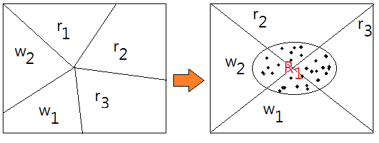
Given that there are 3 red and 2 white balls in a bow. Suppose you pick up 2 balls sequentially. What’s the probability of picking up the 2nd white ball and the 1st one is the red ball?

[Answer]
This is asking for $P(W_{2}\cap R_{1})$. Denote $R_{i}$,$W_{i}$ as the i-th picking the red, white ball up.
➀when we pick up the very first ball, $\Omega$=$\{r_{1},r_{2},r_{3},w_{1},w_{2}\}$.
$P(R_{1})$=$\frac {3}{5}$, the probability that the 1st ball is a red ball.
➁when we pick up the second ball, $\Omega$=$\{r_{2},r_{3},w_{1},w_{2}\}$.
$P(W_{2}\vert R_{1})$=$\frac {2}{4}$, the probability that the 2nd ball is a white ball, given that the first one is the red ball.
➂$P(W_{2}\cap R_{1})$=$P(W_{2}\vert R_{1})\cdot P(R_{1})$=$\frac {6}{20}$.
[More details]
➀$P(R_{1})$ is the prior priority.
➁$P(W_{2}\vert R_{1})$ is the likelihood function to estimate the probability that the 2nd ball is a white ball, given that the first one is the red ball.
➂$P(W_{2}\vert R_{1})\cdot P(R_{1})$ is the joint probability of the coexistence of $W_{2}$ and $R_{1}$, since we are asking for the probability of picking up the 2nd white ball and the 1st one is the red ball.

Example: quantitative versus qualitative::mjtsai1974

[Question]
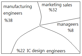
Suppose the statistical population distribution in the Hsin-Chu science park area reports that $\%8$ of the population is the managers, $\%32$ is the marketing sales, $\%38$ is the manufacturing engineers, $\%22$ is the IC design engineers.
Given that Albert is a man, when you see him, his behavior is a little shy, talktive with strangers for road seeking, and is not talktive in political topics.

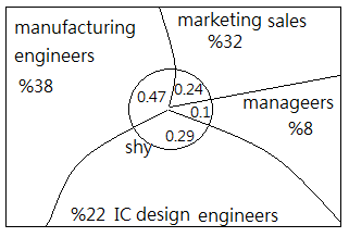
According to recent statistical research that given a manager, $0.1$ probability being shy; given a marketing sales, $0.24$ probability being shy; given a manufacturing engineer, $0.47$ probability being shy; given an IC design engineer, %0.29% probability being shy.
Under such condition, given that Albert is a shy man, what kind of identity has the maximum probability?
[Answer]
➀take $P(Mgr)$=$0.08$, $P(Sales)$=$0.32$, $P(M_{eng})$=$0.38$, $P(I_{eng})$=$0.22$ for probability of being managers, marketing sales, manufacture engineers, IC design engineers, which are all the prior probability.
➁take $P(Shy\vert Mgr)$=$0.1$, $P(Shy\vert Sales)$=$0.24$, $P(Shy\vert M_{eng})$=$0.47$, $P(Shy\vert I_{eng})$=$0.29$ for given a manager, a marketing sales, a manufacturing engineer, IC design engineer, the probability being shy respectively, which are all the likelihood function, the qualitative term.
➂the question asks for the maximum in between $P(Mgr\vert Shy)$, $P(Sales\vert Shy)$, $P(M_{eng}\vert Shy)$, $P(I_{eng}\vert Shy)$. Trivially, we need the total probability of being shy.
$P(Shy)$
=$P(Shy\vert Mgr)\cdot P(Mgr)$+
$\;\;\;\;P(Shy\vert Sales)\cdot P(Sales)$+
$\;\;\;\;P(Shy\vert M_{eng})\cdot P(M_{eng})$+
$\;\;\;\;P(Shy\vert I_{eng})\cdot P(I_{eng})$
=$0.1\cdot 0.08$+$0.24\cdot 0.32$+$0.47\cdot 0.38$+$0.29\cdot 0.22$
=$0.3272$
➃finally, the posterior probability:
$P(Mgr\vert Shy)$=$\frac {P(Shy\vert Mgr)\cdot P(Mgr)}{P(Shy)}$=$\frac {0.1\cdot 0.08}{0.3272}$=$0.0244$
$P(Sales\vert Shy)$=$\frac {P(Shy\vert Sales)\cdot P(Sales)}{P(Shy)}$=$\frac {0.24\cdot 0.32}{0.3272}$=$0.2347$
$P(M_{eng}\vert Shy)$=$\frac {P(Shy\vert M_{eng})\cdot P(M_{eng})}{P(Shy)}$=$\frac {0.47\cdot 0.38}{0.3272}$=$0.5458$
$P(I_{eng}\vert Shy)$=$\frac {P(Shy\vert I_{eng})\cdot P(I_{eng})}{P(Shy)}$=$\frac {0.29\cdot 0.22}{0.3272}$=$0.1949$

By means of quantitative posterior, we found that $P(M_{eng}\vert Shy)$ has the largest posterior probability and implies the maximum possibility that Albert is a shy man, he is a manufacture engineer.

Event Independence versus Conditional Probability

26 May 2018

Prologue To Event Independence versus Conditional Probability

In the disciplines of probability, event independence is quiet an important concept. The inference from conditional probability come out with the result that one event occurrence is said to not related to another event, if the two events are independent.

Definition: Event Independence

An event $A$ is said independent of event $B$, if
$\;\;\;\;P(A\vert B)$=$P(A)$.

Event Independence Equivalence

By the definition of event independence, we can have an equivalence of expression from conditional probability:
$P(A\vert B)$=$\frac {P(A\cap B)}{P(B)}$=$P(A)$
$\Leftrightarrow P(A\cap B)=P(A)\cdot P(B)$

Below lists the basic properties:
➀$P(A\cap B)$=$P(A)\cdot P(B)$ indicates event $A$ is independent of event $B$.
➁by its symmetry, $P(A)\cdot P(B)$=$P(B)\cdot P(A)$=$P(B\cap A)$, event $B$ is independent of event $A$.
➂$P(A\vert B)$=$P(A)$ and $P(B\vert A)$=$P(B)$.

Event Independence Extension

[1] multiple events independence
$P(N_{1}\cap N_{2}\cap…\cap N_{m})$
=$P(N_{1})\cdot P(N_{2})\cdot …\cdot P(N_{m-1})\cdot P(N_{m})$, given that all events $N_{i}$ are all independent.
proof::mjtsai1974
➀$P(N_{m-1}\vert N_{m})$=$\frac {P(N_{m-1}\cap N_{m})}{P(N_{m})}$=$P(N_{m-1})$
Then $P(N_{m-1}\cap N_{m})$
=$P(N_{m-1})\cdot P(N_{m})$.
➁$P(N_{m-2}\vert (N_{m-1}\cap N_{m}))$=$\frac {P(N_{m-2}\cap (N_{m-1}\cap N_{m}))}{P(N_{m-1}\cap N_{m})}$=$P(N_{m-2})$
Then $P(N_{m-2}\cap (N_{m-1}\cap N_{m}))$
=$P(N_{m-2})\cdot P(N_{m-1})\cdot P(N_{m})$.
➂by mathematics induction, could we finally have the equivalence of expression.
[2] independence equivalence relation
Event $A$ is independent of event $B$
$\Leftrightarrow$ event $A^{c}$ is independent of event $B$
proof::mjtsai1974
$1$-$P(A\vert B)$
=$1$-$P(A)$
=$P(A^{c})$
=$P(A^{c}\vert B)$
From the end to the beginning could we prove the inverse direction.
[3] independence of all events
Given event $A$ is independent of event $B$, we can infer out all possible independence in between $A$, $A^{c}$, $B$, $B^{c}$.
proof::mjtsai1974
$P(A\vert B)$=$P(A)$
$\Leftrightarrow P(A^{c}\vert B)$=$P(A^{c})$
$\Leftrightarrow P(B\vert A^{c})$=$P(B)$
$\Leftrightarrow P(B^{c}\vert A^{c})$=$P(B^{c})$
$\Leftrightarrow P(B\vert A)$=$P(B)$
$\Leftrightarrow P(B^{c}\vert A)$=$P(B^{c})$
$\Leftrightarrow P(A\vert B^{c})$=$P(A)$
$\Leftrightarrow P(A^{c}\vert B^{c})$=$P(A^{c})$

We conclude if $A$ is independent of $B$, then $A^{c}$ is independent of $B$, $A$ is independent of $B^{c}$, $A^{c}$ is independent of $B^{c}$.
[4] event and its complemenmt
The prpbability of intersection of any given event and its complement is $0$, that is $P(A\cap A^{c})$=$0$.

Example: 2nd Head following 1st Head

Suppose you are tossing a fair coin, the probability of head and tail are all $\frac {1}{2}$, and each tossing is an independent case.

We’d like to ask for the probability that the 2nd tossing out a head, right after the 1st tossing out a head, then,
➀take the event of 1st tossing as $A_{1}$=$\{H,T\}$, take the event of 2nd tossing as $A_{2}$=$\{H,T\}$.
➁the sample space of these 2 tossing would be $\Omega$=$\{HH,HT,TH,TT\}$. The probability of 2 contiguous heads is $\frac {1}{4}$.
➂the probability that the 2nd tossing out a head, right after the 1st tossing out a head is asking for $P(A_{2}\cap A_{1})$, then
$\frac {1}{4}$
=$P(A_{2}\cap A_{1})$
=$P(A_{2}\vert A_{1})\cdot P(A_{1})$
=$\frac {1}{2}\cdot \frac {1}{2}$
=$P(A_{2})\cdot P(A_{1})$
Thus, we have $P(A_{2}\vert A_{1})$=$P(A_{2})$, it is fully compliant with the given that each tossing is an independent case.

Example: Illustration By Tossing A Fair Die

Suppose you are tossing a fair die, the sample space $\Omega$=$\{1,2,3,4,5,6\}$. We denote the event of numbers smaller than $4$ as $A$=$\{1,2,3\}$, and denote the event of even numbers as $B$=$\{2,4,6\}$.

To evaluate if event $A$ is independent of event $B$:
➀$P(A\cap B)$=$P(\{2\})$=$\frac {1}{6}$
➁$P(A)\cdot P(B)$=$\frac {1}{2}\cdot \frac {1}{2}$=$\frac {1}{4}$
Hence, the event of numbers smaller than $4$ is not independent of the event of even numbers.

Introduction To The Probability

25 May 2018

Prologue To Introduction To The Probability

The probability describes how likely it is the test takes place with the expected result. It is the fundamental for modern world science.

Begin From The Fundamental

[1] sample space
➀sample space is just the set of elements describing the outcomes of the test, experiment, formally, the result after execution of certain action.
In statistics reference text book, the letter $\Omega$ is most often used to represent the sample space.
➁by flipping a coin one time, you will have two outcomes of head and tail, that is to say we associate the sample space with the set $\Omega$=$\{H,T\}$.
➂to guess the birthday within one week, the sample space $\Omega$=$\{Sun,Mon,Tue,Wed,Thu,Fri,Sat\}$.
[2] event
➀subset of a sample space is treated as event.
➁in the birthday in one week example, suppose we’d like to ask for the days with uppercase “S” as the prefix, then, we can denote $S$=$\{Sun,Sat\}$.
➂suppose we’d like to ask for the days with uppercase “T” as the prefix, then, we can denote $T$=$\{Tue,Thu\}$.
[3] intersection, union, complement
Suppose $A$ and $B$ are two events in the sample space $\Omega$.
➀intersection, it’s an event operator, denoted by $\cap$.
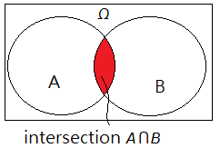➁union, also an event operator, denoted by $\cup$.
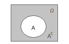
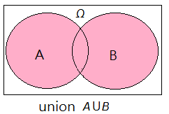➁complement, an event operator, usually denoted by lowercase $c$.

[4] disjoint events
Suppose $A$ and $B$ are two events in the sample space $\Omega$. They are said to be two disjoint events if they have no intersection. $A\cap B$=$0$.
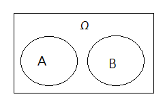Such events might be regarded as mutually exclusive.

The Probability

[1] why do we need the probability?
In order to express how likely it is that an event will occur, during the experiment, by assigning probability to each distinct event would be common. To distribute the probability accurately would not be an easy task.
[2] the probability function
Since each event would be associated with a probability, then we are in need of the probability function.
➀the uppercase “P” is the probability function on a sample space $\Omega$ to assign the event $A$ in $\Omega$ a number $P(A)$ in $[0,1]$. The number $P(A)$ is the probability of the occurrence of event $A$.
➁wherein $P(\Omega)$=$1$
➂$P(A\cup B)$=$P(A)$+$P(B)$-$P(A\cap B)$, where $P(A\cap B)$=$0$ for $A$ and $B$ are disjoint. If $A$,$B$,$C$ are disjoint events, then $P(A\cup B\cup C)$=$P(A)$+$P(B)$+$P(C)$.
[3] the probability is defined on events, not on outcomes
➀tossing a coin one time would we have $\Omega$=$\{H,T\}$, then $P(\{H\})$=$\frac {1}{2}$, $P(\{T\})$=$\frac {1}{2}$, under the assumption that head and tail chances are coming to an equilibrium.
➁given cards of read, blue, green colours. The permutation of all the possible orders of cards would be $\Omega$=$\{RGB$,$RBG$,$GRB$,$GBR$,$BRG$,$BGR\}$.
$P(\{RGB\})$=$P(\{RBG\})$=$P(\{GRB\})$=$P(\{GBR\})$=$P(\{BRG\})$=$P(\{BGR\})$=$\frac {1}{6}$…the same probability for each distinct event.
➂the same example as above, the probability of the event that green card is in the middle would be $P(\{RGB,BGR\})$=$\frac {1}{3}$.
The $\{RGB,BGR\}$ is such event we desire, wherein the $\{RGB\}$ and $\{BGR\}$ are the outcomes described by $\Omega$.
[4] additivity of probability
➀using the same card example, the probability of the event that green card is in the middle could be $P(\{XGX\})$=$P(\{RGB\})$+$P(\{BGR\})$=$\frac {1}{3}$.
This implies that the probability of an event could be obtained by summing over the probabilities of the outcomes belonging to the same event.
➁given $A$ is an event, then $P(A)$+$P(A^{c})$=$P(\Omega)$=$1$.
➂if $A$, $B$ are not disjoint, then $A$=$(A\cap B)\cup(A\cap B^{c})$, this is a disjoint union.
Therefore, $P(A)$=$P(A\cap B)$+$P(A\cap B^{c})$.

Product Of Sample Space

[1] run the same test over multiple times
To justify the experiment result, one single test would be executed over multiple times.
➀suppose we flip the same coin over 2 times, the sample space $\Omega$=$\{H,T\}$x$\{H,T\}$.
It is now $\Omega$=$\{HH,HT,TH,TT\}$. Total 4 outcomes in it, we can take one outcome as one event, then $P(\{HH\})$=$P(\{HT\})$=$P(\{TH\})$=$P(\{TT\})$=$\frac {1}{4}$, under the assumption that $P(\{H\})$=$P(\{T\})$ in each single tossing of coin.
[2] combine the sample space from different tests
➀given that 2 sample spaces with respect to 2 different tests’ outcomes, they are $\Omega_{1}$,$\Omega_{2}$, where sizeof($\Omega_{1}$)=$r$, sizeof($\Omega_{2}$)=$s$.
➁then $\Omega$=$\Omega_{1}$x$\Omega_{2}$, sizeof($\Omega$)=$r\cdot s$. If we treat each distinct combination in the sample space as one single event, the probability of such distinct event is $\frac {1}{r\cdot s}$. The $\frac {1}{r}$,$\frac {1}{s}$ are the probability for the occurrences of outcomes in the $\Omega_{1}$ and $\Omega_{2}$ with respect to test 1 and test 2.
[3] general form of the same test over multiple times
➀suppose we’d like to make the experiment for n runs. We take $\Omega_{i}$ to be the sample space of the i-th test result, $\omega_{i}$ to be one of the outcomes in $\Omega_{i}$.
➁if the occurrence of each outcome $\omega_{i}$ has probability $p_{i}$, then $P(\{\omega_{1},\omega_{2}…\omega_{n}\})$=$p_{1}\cdot p_{2}…p_{n}$, which is the probability for the event $\{\omega_{1},\omega_{2}…\omega_{n}\}$ to take place.
➂assume we flip a coin with probability $p$ of head, that implies $1-p$ of tail. Then the probability of 1 single head after 4 times of tossing would be $4\cdot (1-p)^3\cdot p$.
The sample space would be
$\Omega$=$\{(HTTT),(THTT),(TTHT),(TTTH)\}$. There are 4 combinations, with each has probability $(1-p)^{3}\cdot p$.

An Infinite Sample Space

[1] run the same test until succeeds
➀suppose we’d like to toss a coin until it appears with head. If the tail is always the result, the sample space $\Omega$=$\{T_{1},T_{2},T_{3},…,T_{n}…\}$, $n\rightarrow\infty$.
Next to ask the probability function of this sample space. Assume the probability of head is $p$, the tail is $1-p$.
[2] run the same test until succeeds
➀for the simplicity, we’d like to change the notation by $\Omega$=$\{1,2,..,n,…\}$ for the number of iterations the tossing coin result coming out with a head.
➁$P(1)$=$P(\{H\})$=$p$
➂$P(2)$=$P(\{TH\})$=$(1-p)\cdot p$
➃$P(n)$=$P(\{T_{1}T_{2}…T_{n-1}H_{n}\})$=$(1-p)^{n-1}\cdot p$
➄when $a$ is incredibly large, the total probability becomes
$\lim_{n\rightarrow\infty}P(1)+P(2)+…+P(n)$
=$\lim_{n\rightarrow\infty}p+(1-p)\cdot p+…+(1-p)^{n-1}\cdot p$
=$\lim_{n\rightarrow\infty}p\cdot\frac {1}{1-(1-p)}$
=$p\cdot\frac {1}{p}$
=$1$…the total probability

In an infinite sample space, if all the events $A_{1}$,$A_{2}$,…,$A_{n}$ are disjoint, then,
$P(\Omega)$
=$P(A_{1}\cup A_{2}\cup…\cup A_{n})$
=$P(A_{1})$+$P(A_{2})$+…$P(A_{n})$
=$1$

Introduction To The Conditional Probability

25 May 2018

Prologue To Introduction To The Conditional Probability

Based on the probability of some already occurred event, we can infer or reassess the probability of another event, which is the major effect of the conditional probability.

Definition: Conditional Probability

Given the probability $P(C)$ of the already occurred event $C$, we can compute another event $A$’s probability $P(A\vert C)$. The conditional probability is defined:
$\;\;\;\;P(A\vert C)$=$\frac {P(A\cap C)}{P(C)}$, provided that $P(C)>0$.

This implies that the conditonal probability could help to find out the fraction of the probability of event $C$ is also in event $A$, which is $P(A\cap C)$.

Conditional Probability Properties

Given that $P(C)>0$, we can deduce out below properties:
➀$P(A\vert C)$+$P(A^{c}\vert C)$=$1$, holds for all conditions.
➁if $A\cap C$=$0$, then $P(A\vert C)$=$0$.
➂if $C\subset A$, then $A\cap C$=$C$, $P(A\vert C)$=$1$.
➃if $A\subset C$, then $A\cap C$=$A$, $P(A\vert C)$=$\frac {P(A)}{P(C)}\ge P(A)$, since $P(C)\le 1$.

Example: Illustration By Tossing A Fair Die

Suppose you are tossing a fair die, the sample space $\Omega$=$\{1,2,3,4,5,6\}$. We denote the event of numbers smaller than $3$ as $A$=$\{1,2\}$, and denote the event of even numbers as $B$=$\{2,4,6\}$.
➀if we know the current rolled out number is even, what’s the probability the number is smaller than $3$?
$P(A\vert B)$=$\frac {P(A\cap B)}{P(B)}$=$\frac {\frac {1}{6}}{\frac {1}{2}}$=$\frac {1}{3}$,
where $P(A\cap B)$=$P(\{2\})$=$\frac {1}{6}$.
➁if we know the rolled out number is smaller than $3$, what’s the probability the number is even?
$P(B\vert A)$=$\frac {P(B\cap A)}{P(A)}$=$\frac {\frac {1}{6}}{\frac {1}{3}}$=$\frac {1}{2}$.

Example: Illustration By Fuel Residence Time

Given a engine full of chemical fuel in its combustion chamber and just starts, we denote the event that the particle is left as non-comleted chemical reaction state after t seconds as $R_{t}$.

Suppose the probability of such chemical reaction is in exponential distribution, the probability of $R_{t}$, $P(R_{t})$=$e^{-t}$.

Then, the probability of the particle stay over 4 seconds will stay over 5 seconds would be to ask for $P(R_{5}\vert R_{4})$.
➀$R_{4}$=$e^{-4}$
➁$R_{5}$=$e^{-5}$
➂since $R_{5}\subset R{4}$, we have $R_{5}\cap R_{4}$=$R_{5}$.
Therefore, $P(R_{5}\vert R_{4})$=$\frac {P(R_{5}\cap R_{4})}{P(R_{4})}$=$\frac {P(R_{5})}{P(R_{4})}$=$e^{-1}$.

The Probability Chaining Rule

The probability chaining rule has it that:
➀$P(A\cap C)=P(A\vert C)\cdot P(C)$
➁$P((A\cap B)\vert C)$=$P(A\vert (B\cap C))\cdot P(B\vert C)$
➂$P(A\cap B\cap C)$=$P(A\vert (B\cap C))\cdot P(B\vert C)\cdot P(C)$
proof::mjtsai1974
➀begin from the conditional probability:
$P(A\vert C)$=$\frac {P(A\cap C)}{P(C)}$
$\Leftrightarrow P(A\cap C)=P(A\vert C)\cdot P(C)$
➁$P((A\cap B)\vert C)$
=$\frac {P((A\cap B)\cap C)}{P(C)}$
=$\frac {P(A\cap (B\cap C))}{P(C)}$
=$\frac {P(A\vert (B\cap C))\cdot P(B\cap C)}{P(C)}$
=$P(A\vert (B\cap C))\cdot P(B\vert C)$
➂from above,
$\frac {P((A\cap B)\cap C)}{P(C)}$=$P(A\vert (B\cap C))\cdot P(B\vert C)$
$\Leftrightarrow P(A\cap B\cap C)$=$P(A\vert (B\cap C))\cdot P(B\vert C)\cdot P(C)$

Also known as the multiplication rule.
Below expression illustrates probability chaining rule extension:
$P(N_{1}\cap N_{2}\cap N_{3}\cap …\cap N_{m})$
=$P(N_{1}\vert (N_{2}\cap N_{3}\cap …\cap N_{m}))$
$\;\;\;\;\cdot P(N_{2}\vert (N_{3}\cap …\cap N_{m}))$
$\;\;\;\;...$
$\;\;\;\;\cdot P(N_{m-1}\vert N_{m})$
$\;\;\;\;\cdot P(N_{m})$

Example: Illustration By Fuel Residence Time For Extension

If we are given the same condition to the engine containing a combustion chamber in it, we’d like to estimate the probability of the particle stay over 1 seconds will stay over 10 seconds.
Suppose the chemical particle still left at 10-th second is the final one molecular.
And the probability of such chemical reaction is in exponential distribution, the probability of $R_{t}$, $P(R_{t})$=$e^{-t}$.
proof::mjtsai1974
This is to ask for $P(R_{10}\vert R_{1})$=$\frac {P(R_{10}\cap R_{1})}{P(R_{1})}$.
➀by the given assumption, the final particle is in $R_{10}$, it just passed through $R_{1}$,$R_{2}$,...,$R_{10}$.
Hence, $(R_{10}\cap R_{1})$=$(R_{10}\cap R_{9}\cap … \cap R_{1})$
➁by the probability chaining rule,
$P(R_{10}\cap R_{9}\cap … \cap R_{1})$
=$P(R_{10}\vert (R_{9}\cap … \cap R_{1}))$
$\;\;\;\;\cdot P(R_{9}\vert (R_{8}\cap … \cap R_{1}))$
$\;\;\;\;\cdot P(R_{8}\vert (R_{7}\cap … \cap R_{1}))$
$\;\;\;\;…$
$\;\;\;\;\cdot P(R_{3}\vert (R_{2}\cap R_{1}))$
$\;\;\;\;\cdot P(R_{2}\vert R_{1})$
$\;\;\;\;\cdot P(R_{1})$
➂with each multiplication term equaling to $e^{-1}$,
$P(R_{10}\cap R_{9}\cap … \cap R_{1})$=$e^{-10}$
then, $P(R_{10}\vert R_{1})$=$\frac {P(R_{10}\cap R_{1})}{P(R_{1})}$=$e^{-9}$.

Introduction To The Bayes Theorem

23 May 2018

Prologue To Introduction To The Bayes Theorem

The Bayes theorem has been developed and evolved over time to enhance the accuracy of conditional probability prediction result, especially, when you have only a few data gathered and would like to have a convincible, plausible result. It could be pervasively found in the machine learning, reinforcement learning, wherein the POMDP transition probability is one such model.

Law Of Total Probability

Consider in a random experiment, given below conditions:
➀$\Omega$=$\{B_{1},B_{2},…,B_{n}\}$, where $B_{i}\cap B_{j}$=$0$.
➁within the sample space, there exist another event $A$, partitioned by $B_{i}$ randomly.
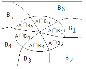We have $P(A)$=$P(A\vert B_{1})\cdot P(B_{1})$+…+$P(A\vert B_{n})\cdot P(B_{n})$

proof:
➀by intersection of $A$ and $\Omega$ could we get $A$:
$A$
=$A\cap \Omega$
=$A\cap (B_{1}\cup B_{2}\cup…\cup B_{n})$
=$(A\cap B_{1})\cup (A\cap B_{2})…\cup (A\cap B_{n})$.
➁the total probability of event $A$:
$P(A)$
=$P((A\cap B_{1})\cup (A\cap B_{2})…\cup (A\cap B_{n}))$
=$P(A\cap B_{1})$+$P(A\cap B_{2})$+…+$P(A\cap B_{n})$
=$P(A\vert B_{1})\cdot P(B_{1})$+…+$P(A\vert B_{n})\cdot P(B_{n})$